Chapter 3 Processing
In this final section of this short book, we will address how to process postural data. So far, we have managed (i.e., merged data, synthetised data) and pre-processed (i.e., apply filters) postural data. Now we want to process the data.
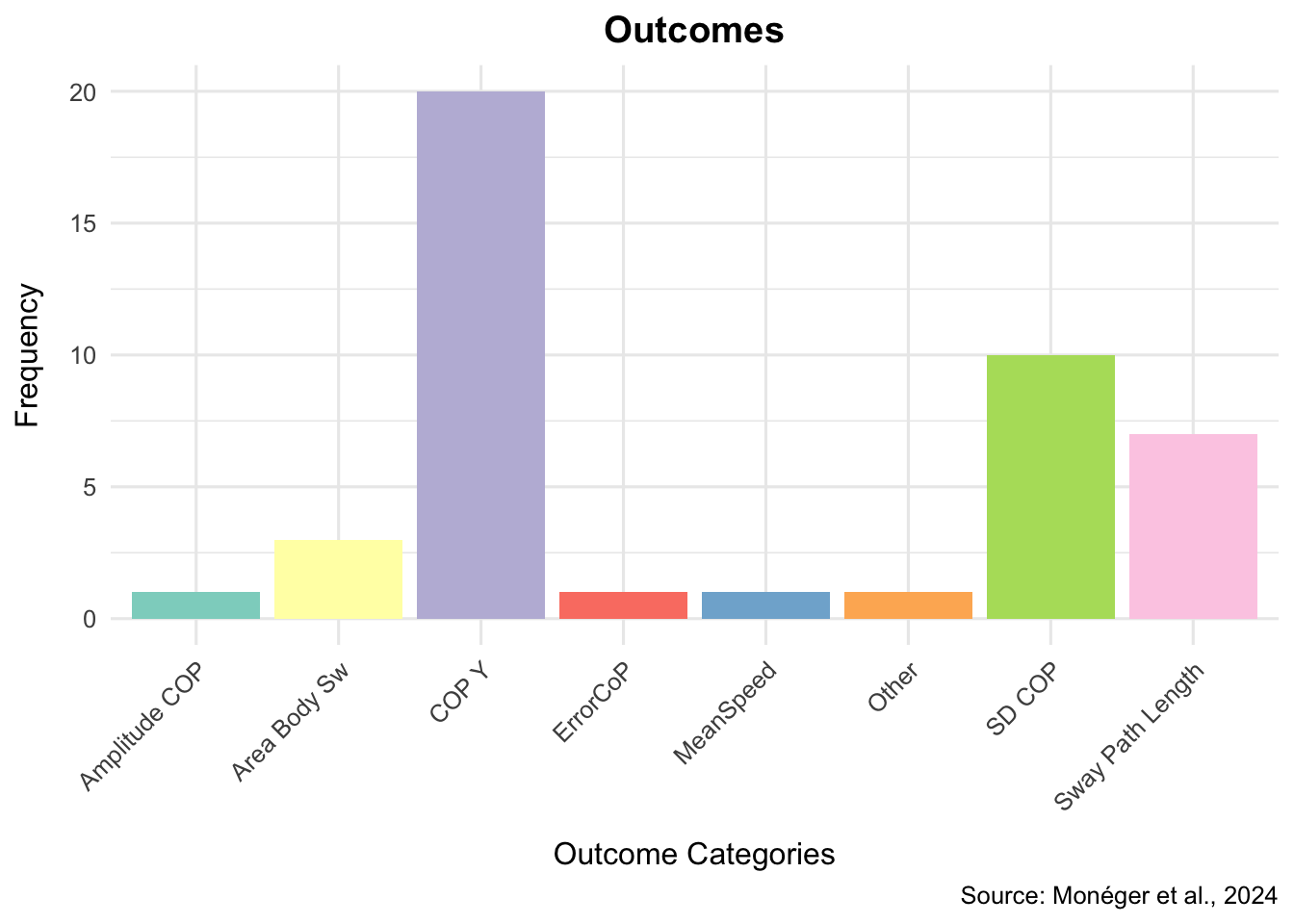
By postural data processing, the author means: computing the type(s) of postural indicator that you might be interested in. Indeed, the postural field is plagued with more than 400 possible postural indicators. Some of these are highly popular (e.g., CoP-Y, SD CoP-X, Sway Path Length), while others might be more obscure (e.g., Root Mean Square radius, Fractal dimension, set of zero-crossings). In their meta-analysis, Monéger et al. (2024 [preprint]) assessed the different indicators used in the literature that targeted postural approach and avoidance of pleasant and unpleasant stimuli. Their review indicated that no less than 8 different indicators could be counted (after some re-arranging to account for authors using different terms to measure the same thing): average CoP displacements, deviations of average CoP from a baseline, Amplitude of CoP displacements, Standard deviations of CoP displacements (SD CoP), Sway Path Length, Area of body sway, Mean Speed of CoP displacements, and other unique concepts (e.g., rambling/trembling components of body sway). Importantly, it is possible to classify the indicators in two categories:
- indicators that evaluate absolute displacement (e.g., CoP, or maximum CoP displacement)
- indicators that evaluate variability in CoP displacements (e.g., Standard deviation of CoP displacements, 95% confidence elipse area, etc.)
The former category should be of interest to researcher who wants to evaluate approach and avoidance, whereas the latter category is of interest to researchers who want to study freezing or loss of stability. Whereas for approach and avoidance, CoP displacements on the antero-posterior axis are close to be the only variable available; when it comes to freezing indicators, there is a large number of possible measures. Fortunately, some or more popular than others, and a possible standardisation toward sway path length and standard deviations of CoP displacements seems likely in the future (see Figure X).
Figure X. Distribution of the different postural indicators in the field.
The BalanceMate package provides reader with tools to easily compute: CoP (on the X and/or Y axes), Sway Path Length, x% Confidence Elipse Area, and Standard Deviation of CoP (on the X and/or Y axes). To be sure, other indicators exist - albeit they might be less frequent. It is not impossible that future versions of the package integrate some of these measures. However, it is the authors’ personal view that the heterogeneity in data processing constitutes a problem in the field. Thus reducing the possibilities to the most popular choices might be a good thing. Here also, transparency (and possibly registration) are key to avoid the pitfalls of excessive undisclosed flexibility (a.k.a., p-hacking).
In addition to enabling the easy computation of postural indicators, the BalanceMate package also provides visualisation of the so-called “spaghetti” plot.
3.1 Computations
The BalanceMate package provides specific commands to compute specific postural indicators (e.g., CoPX_ComputeR, EllipseArea_ComputeR). However, it provides a very useful wrapper that can also compute any postural indicator, provided you use the “indicator” argument correctly. In the following subsections, we will review the different commands. All of them follow a similar syntax, with the same arguments (with very few exceptions): they require:
- the base columns (most of the time, the CoP column, but sometimes – for instance when computing the CoP itsel – it might require forces and moments),
- the time bin of interest (most measures, with the exception of the CoP, being variability measures, they requires a time bin specification - should the readers be interested in computing the indicator at the participant level, they should write a time bin size equal to the protocol duration [minus possible periods that does not interest them and that were previously removed, see Chapter 1]),
- the sample rate used in the protocol.
To illustrate each command, we’ll go back to where we left: D’Api and De Reinette ran their study, the pre-processed the signal, and now they want to compute some postural indicators. They registered that they would analyse all indicators covered by the BalanceMate package.
library(BalanceMate)

Data<-Merge_PosData("~/Desktop/BalanceMate/inst/extdata/", SampleRate = 100, SessionDuration = 100)
filtered_data <- Butterworth_it(
  Data = Data,
  cutoff_freq = 5,
  filter_order = 2,
  sampling_rate = 100,
  type = "low",
  Colname = c("CoP_X", "CoP_Y")
)

# Identify the time cuts in your protocol:
cuts<-c(20,
                     22,
                     30,
                     32,
                     40,
                     42,
                     50,
                     52,
                     60,
                     62,
                     70,
                     72,
                     80,
                     82,
                     90,
                     92)

# Label the periods:
Label = c("Training",
          "Fix",
          "Trial_1",
          "Fix",
          "Trial_2",
          "Fix",
          "Trial_3",
          "Fix",
          "Trial_4",
          "Fix",
          "Trial_5",
          "Fix",
          "Trial_6",
          "Fix",
          "Trial_7",
          "Fix",
          "Trial_8")


Annotated_Data <- Time_StampeR(df = Data, id_col = "file_name", sample_rate = 100, protocol_duration = 100, cuts = cuts, period_names = Label)

Data <- subset(Annotated_Data, Annotated_Data$Period_Name != "Blank" & Annotated_Data$Period_Name != "Fix")
CoPX_ComputeR
A function to compute CoP-X. Requires a data frame containing 1) moments on the Y axis, and 2) Forces on the z-axis.
Note that because the Merge_PosData command already computes CoP X and CoP Y by default, it is redundant to compute those indicators again, but we’ll do it here for the sake of example)
(Note also that although counter-intuitive, CoP-X computation is performed using My, and CoP-Y computation is performed using Mx)
##        Fx      Fy       Fz      Mx      My       Mz Time          file_name      CoP_X
## 1 7.24049 7.22547 790.0556 5.47499 7.68121 -0.16553 0.00 Postural_DataA.txt -0.9722367
## 2 7.46415 7.30759 789.6346 5.41001 7.61477 -0.14419 0.01 Postural_DataA.txt -0.9643410
## 3 7.80475 7.35250 789.3054 5.34504 7.54834 -0.12477 0.02 Postural_DataA.txt -0.9563269
## 4 7.60925 7.46016 789.3280 5.34504 7.54834 -0.16260 0.03 Postural_DataA.txt -0.9562995
## 5 7.49666 6.98660 788.6198 5.34434 7.41616 -0.02562 0.04 Postural_DataA.txt -0.9403974
## 6 7.42719 6.95055 788.2588 5.27937 7.34973 -0.07609 0.05 Postural_DataA.txt -0.9324006
##       CoP_Y Period_Name    CoPXnew
## 1 0.6929880    Training -0.9722367
## 2 0.6851283    Training -0.9643410
## 3 0.6771827    Training -0.9563269
## 4 0.6771634    Training -0.9562995
## 5 0.6776827    Training -0.9403974
## 6 0.6697508    Training -0.9324006
CoPY_ComputeR
A function to compute CoP-Y. Requires a data frame containing 1) moments on the X axis, and 2) Forces on the z-axis. note: although counterintuitive, CoP-Y is derived from the inverse rotation of the X axis (moment) - inverse because of conventions.
Because D’Api and De Reinette are interested in approach and avoidance of pictures of planes, they should be particularly interested in the CoP-Y.
##        Fx      Fy       Fz      Mx      My       Mz Time          file_name      CoP_X
## 1 7.24049 7.22547 790.0556 5.47499 7.68121 -0.16553 0.00 Postural_DataA.txt -0.9722367
## 2 7.46415 7.30759 789.6346 5.41001 7.61477 -0.14419 0.01 Postural_DataA.txt -0.9643410
## 3 7.80475 7.35250 789.3054 5.34504 7.54834 -0.12477 0.02 Postural_DataA.txt -0.9563269
## 4 7.60925 7.46016 789.3280 5.34504 7.54834 -0.16260 0.03 Postural_DataA.txt -0.9562995
## 5 7.49666 6.98660 788.6198 5.34434 7.41616 -0.02562 0.04 Postural_DataA.txt -0.9403974
## 6 7.42719 6.95055 788.2588 5.27937 7.34973 -0.07609 0.05 Postural_DataA.txt -0.9324006
##       CoP_Y Period_Name    CoPXnew   CoPYnew
## 1 0.6929880    Training -0.9722367 0.6929880
## 2 0.6851283    Training -0.9643410 0.6851283
## 3 0.6771827    Training -0.9563269 0.6771827
## 4 0.6771634    Training -0.9562995 0.6771634
## 5 0.6776827    Training -0.9403974 0.6776827
## 6 0.6697508    Training -0.9324006 0.6697508
SPL_ComputeR
A function that computes Sway Path Length. You will need a data frame containing: 1) a unique session/participant identifier, 2) CoP-X, 3) CoP-Y, and optionnally to compute indicators per epoch, 4) a time column, 5) a specification of an epoch (e.g. 1 second).
Here, as already stated, De Reinette & D’api are interested in synthetising their data into 1s time bins. The resulting object will thus be a shorter data frame (our 162000 rows-long data frame will shrink to a 1620 rows data frame). Thus, in contrast to the two aforementionned command that output a vector of the same lenght as the initial dataframe, the following commands using epochs will output dataframes
Note however that, should you not indicate any Time column and epoch lenght, the output will be a data frame where the indicators would be computed at the participant level.
Data_SPL <- SPL_ComputeR(Data,
                         CoPX_col = "CoP_X",
                         CoPY_col = "CoP_Y",
                         ID = "file_name",
                         time_col = "Time",
                         epoch_length = 1)

head(Data_SPL)
## participant_id epoch sway_path_length
## Postural_DataA.txt.1 Postural_DataA 1 1.625021
## Postural_DataA.txt.2 Postural_DataA 2 1.568201
## Postural_DataA.txt.3 Postural_DataA 3 2.521197
## Postural_DataA.txt.4 Postural_DataA 4 1.537481
## Postural_DataA.txt.5 Postural_DataA 5 2.006376
## Postural_DataA.txt.6 Postural_DataA 6 1.334722EllipseArea_ComputeR
A function that computes the X percent confidence interval area. You will need a data frame containing: 1) a unique session/participant identifier, 2) CoP-X, 3) CoP-Y, and optionnally to compute indicators per epoch, 4) a time column, 5) a specification of an epoch (e.g. 1 second). Optionally, you can specify which type of confidence you want for that ellipse – the default is 95%.
Data_Area <- compute_ellipse_area(Data,
                                  CoPX_col = "CoP_X",
                                  CoPY_col = "CoP_Y",
                                  ID = "file_name",
                                  time_col = "Time",
                                  epoch_length = 1)

head(Data_Area)
## participant_id epoch ellipse_area
## Postural_DataA.txt.1 Postural_DataA 1 0.2931300
## Postural_DataA.txt.2 Postural_DataA 2 0.2275301
## Postural_DataA.txt.3 Postural_DataA 3 0.6424802
## Postural_DataA.txt.4 Postural_DataA 4 0.2057300
## Postural_DataA.txt.5 Postural_DataA 5 1.0342947
## Postural_DataA.txt.6 Postural_DataA 6 0.1943726SD_CoP_ComputeR
A function that computes the standard deviation of the CoP-X and CoP-Y movements. You will need a data frame containing: 1) a unique session/participant identifier, 2) CoP-X, 3) CoP-Y, and optionnally to compute indicators per epoch, 4) a time column, 5) a specification of an epoch (e.g. 1 second).
Data_SD <- SD_CoP_ComputeR(Data,
                                  CoPX_col = "CoP_X",
                                  CoPY_col = "CoP_Y",
                                  ID = "file_name",
                                  time_col = "Time",
                                  epoch_length = 1)

head(Data_SD)
## participant_id epoch SD_CoPX SD_CoPY
## Postural_DataA.txt.1 Postural_DataA 1 0.17386750 0.2564255
## Postural_DataA.txt.2 Postural_DataA 2 0.06674033 0.1832425
## Postural_DataA.txt.3 Postural_DataA 3 0.06926711 0.6096262
## Postural_DataA.txt.4 Postural_DataA 4 0.04483301 0.2625958
## Postural_DataA.txt.5 Postural_DataA 5 0.13179252 0.4427927
## Postural_DataA.txt.6 Postural_DataA 6 0.08765722 0.1496152All these specific commands are of interests. However, BalanceMate also provide a wrapper that might be of interest to facilitate computations.
The Compute_Postural_Indicators is a flexible way of computing one or multiple indicators. It is also very straightforward to use, as it requires the same elements as the other functions (with optionnal argument for the confidence in case you use the elipse area):
CompleteData <- compute_postural_indicators(Data, CoPX_col = "CoP_X", CoPY_col = "CoP_Y", ID = "file_name", time_col = "Time", epoch_length = 1, indicators = c("CoP_X", "CoP_Y", "SwayPathLength", "EllipseArea", "SD_CoP_X", "SD_CoP_Y"))

head(CompleteData)
## participant_id epoch CoP_X CoP_Y SwayPathLength EllipseArea SD_CoP_X
## 1 Postural_DataA 1 -0.7024449 0.8916070 1.625021 0.2931300 0.17386750
## 13 Postural_DataA 2 -0.5186725 0.7656363 1.568201 0.2275301 0.06674033
## 22 Postural_DataA 3 -0.6890181 2.1369338 2.521197 0.6424802 0.06926711
## 31 Postural_DataA 4 -0.4029652 1.9005180 1.537481 0.2057300 0.04483301
## 40 Postural_DataA 5 -0.7052528 1.0709691 2.006376 1.0342947 0.13179252
## 49 Postural_DataA 6 -0.4380722 0.2547817 1.334722 0.1943726 0.08765722
## SD_CoP_Y
## 1 0.2564255
## 13 0.1832425
## 22 0.6096262
## 31 0.2625958
## 40 0.4427927
## 49 0.1496152Because of its flexibility, this command will be a great tool for researchers interested in computing flexibly multiple indicators.
3.2 Visualise
Finally, the BalanceMate package offers the possibility of visualising samples of your data under the form of “spaghetti plots”. This type of visual representation of postural data can be particularly interesting for researchers wanting to illustrate postural measures, or for case analysis. It can however also be used for giving an average body sway across trials and/or participants.
3.2.1 SpaghettEllipse : Plot sample data
SpaghettEllipse(Data, participant_id_col= "file_name", participant_id = "Postural_DataA.txt", time_col = "Time", time_start = 10, time_end = 60, copx_col = "CoP_X", copy_col = "CoP_Y", Title = "Spaghetti plot for 50 seconds of trial of Participant A" )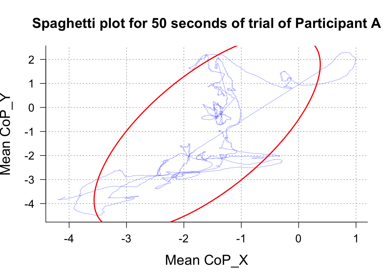
3.2.2 Exploring some possibilities for visualisation
plotting a sample of postural data is interesting. However, maybe readers are interested in some visualisation of average displacements over time. For instance, D’Api and De Reinette might want to plot the average displacements in “Plane” vs “Bikes” conditions.
We can use the Spaghett function to do this. It will require, however, a little bit of brain-poking. So we might want to go back to the “Managing” section of the book.
In our base data frame, we have a unique participant identifier (file_name), and a Time flow column. Usually, we would use synthetise the data at a specific time interval (epoch). However, to enable the visualisation of the average body sway across participants, we can synthetise data for each sample collected across participants - that is, we will use the Time column as an Identifier.
So first: We compute average CoP X and CoP-Y for each “time sample” regardless of participant’s unique identifier:
PartipantLevel<-compute_postural_indicators(Data, CoPX_col = "CoP_X", CoPY_col = "CoP_Y", ID = "Time", indicators = c("CoP_X", "CoP_Y"))And then we can use our Spaghetti plot (Note that the output indicate that our time flow measure is a “participant_id” – but don’t be fooled, it is indeed our time flow, we just tricked the command into thinking it was a participant’s unique identifier):
PartipantLevel$participant_id <- as.numeric(PartipantLevel$participant_id)

PartipantLevel <- PartipantLevel[order(PartipantLevel$participant_id),]
SpaghettEllipse(PartipantLevel, copx_col = "CoP_X", copy_col = "CoP_Y", time_col = "participant_id")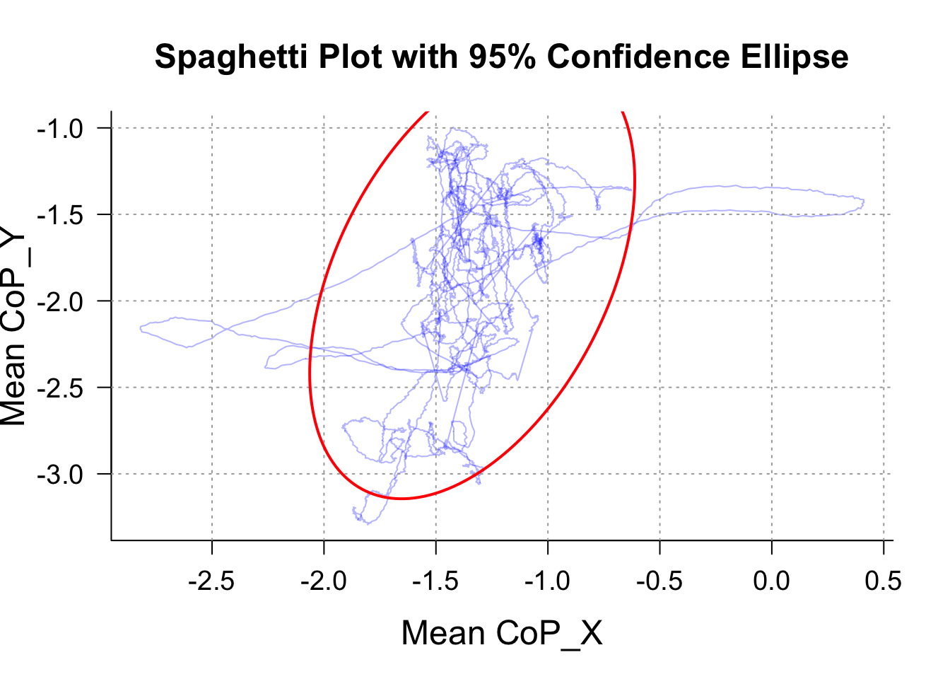
Neat. However, this is the average Spaghetti across participants throughout the session. This is not very informative to D’Api and De Reinette. Surely they would prefer having a visualisation of the body sway across participants for each trials in a specific condition.
Here, we assume that you annotated your Data using the Time_StampeR. We can thus say that the trial type is our unique identifier. For the sake of the example, let’s assume that we know that each odd trial is a Plane, and each even number is a Bike. We can use our time Stamper to indicate it:
Data<-Merge_PosData("~/Desktop/BalanceMate/inst/extdata/", SampleRate = 100, SessionDuration = 100)
filtered_data <- Butterworth_it(
  Data = Data,
  cutoff_freq = 5,
  filter_order = 2,
  sampling_rate = 100,
  type = "low",
  Colname = c("CoP_X", "CoP_Y")
)
# Identify the time cuts in your protocol:
cuts<-c(20,
                     22,
                     30,
                     32,
                     40,
                     42,
                     50,
                     52,
                     60,
                     62,
                     70,
                     72,
                     80,
                     82,
                     90,
                     92)

# Label the periods:
Label = c("Training",
          "Fix",
          "Bike",
          "Fix",
          "Plane",
          "Fix",
          "Bike",
          "Fix",
          "Plane",
          "Fix",
          "Bike",
          "Fix",
          "Plane",
          "Fix",
          "Bike",
          "Fix",
          "Plane")


Annotated_Data <- Time_StampeR(filtered_data, id_col = "file_name", sample_rate = 100, protocol_duration = 100, cuts = cuts, period_names = Label)

head(Annotated_Data)
## Fx Fy Fz Mx My Mz Time file_name CoP_X
## 1 7.24049 7.22547 790.0556 5.47499 7.68121 -0.16553 0.00 Postural_DataA.txt -0.9722367
## 2 7.46415 7.30759 789.6346 5.41001 7.61477 -0.14419 0.01 Postural_DataA.txt -0.9643410
## 3 7.80475 7.35250 789.3054 5.34504 7.54834 -0.12477 0.02 Postural_DataA.txt -0.9563269
## 4 7.60925 7.46016 789.3280 5.34504 7.54834 -0.16260 0.03 Postural_DataA.txt -0.9562995
## 5 7.49666 6.98660 788.6198 5.34434 7.41616 -0.02562 0.04 Postural_DataA.txt -0.9403974
## 6 7.42719 6.95055 788.2588 5.27937 7.34973 -0.07609 0.05 Postural_DataA.txt -0.9324006
## CoP_Y CoP_X_filtered CoP_Y_filtered Period_Name
## 1 0.6929880 -0.5296359 0.3769837 Training
## 2 0.6851283 -0.6285757 0.4463873 Training
## 3 0.6771827 -0.7166685 0.5076296 Training
## 4 0.6771634 -0.7903816 0.5581187 Training
## 5 0.6776827 -0.8486863 0.5970532 Training
## 6 0.6697508 -0.8922511 0.6248892 TrainingWe only keep trials of interest (planes and bikes; getting rid of fixation crosses, training trials and blanks)
BikeData<-subset(Annotated_Data, Annotated_Data$Period_Name == "Bike")

PlaneData<-subset(Annotated_Data, Annotated_Data$Period_Name == "Plane")
We now have two data frames: one that contains all Bike trials of all participants, and another that contains all Plane trials of all participants.
Let’s – just this once – use base R instead of the package. We know each trial is 8 second long. Let’s just manually stamp time in the most straightforward manner:
BikeData$Time <- rep(seq(0.01, 8, by = 0.01), times = 6 * 4) # 6 participants, 4 trials, timed from 0.01 to 8s

PlaneData$Time <- rep(seq(0.01, 8, by = 0.01), times = 6 * 4) # 6 participants, 4 trials, timed from 0.01 to 8s
Now we can compute Mean CoP-X and CoP-Y for each time stamp (e.g., 0.01, 0.02, 0.03, etc.) across participants.
BikeTrialLevel<-compute_postural_indicators(BikeData, CoPX_col = "CoP_X_filtered", CoPY_col = "CoP_Y_filtered", ID = "Time", indicators = c("CoP_X", "CoP_Y")) ### A tester.

PlaneTrialLevel<-compute_postural_indicators(PlaneData, CoPX_col = "CoP_X_filtered", CoPY_col = "CoP_Y_filtered", ID = "Time", indicators = c("CoP_X", "CoP_Y")) ### A tester.
Now, we have two data frames:
One contain the average CoP displacements across participants and trials in the Bike condition
One contain the average CoP displacements across participants and trials in the Plane condition
Note that the time variable is written under “participant_id” because we used time as a grouping variable in our last time_stampeR call.
Let’s plot these:
SpaghettEllipse(BikeTrialLevel, time_col = "participant_id", Title = "Average CoP displacements | bike condition")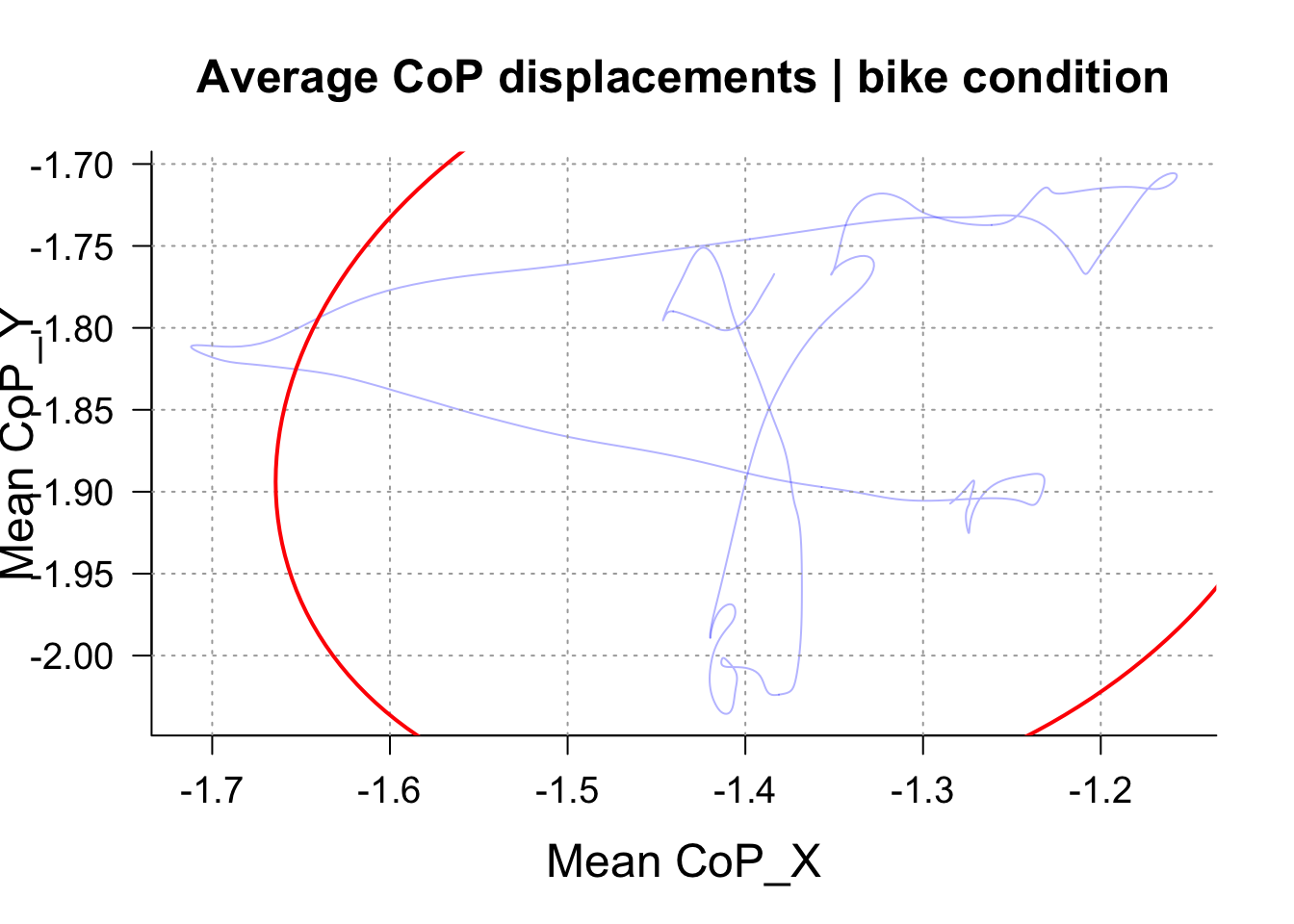
SpaghettEllipse(PlaneTrialLevel, time_col = "participant_id", Title = "Average CoP displacements | Plane condition")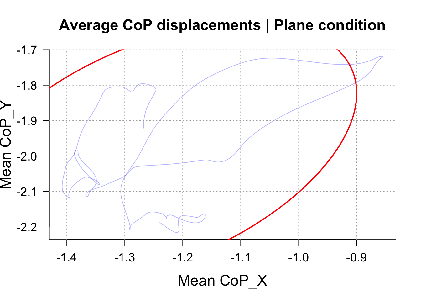
Note: because we are using toy data with only 6 participants and only 64 seconds of recording for each participants, and that the trial plotted is only 8seconds long, the sway path lenght is pretty short, but also pretty noisy. Hopefully this will look better with your data.