Chapter 2 Pre-Processing

Signals can be messy. Indeed, let’s take a look at some samples of the raw postural data that was measured by D’Api and De Reinette in their study:

install.packages("/Users/sylviemoneger/Desktop/BalanceMate_0.0.0.9000.tar.gz", repos = NULL, type = "source")

library(BalanceMate)

Data<-Merge_PosData("~/Desktop/BalanceMate/inst/extdata/", SampleRate = 100, SessionDuration = 100)

plot(x = subset(Data, Data$file_name == "Postural_DataC.txt" & Data$Time > 30 & Data$Time < 32)$Time, 
     y = subset(Data, Data$file_name == "Postural_DataC.txt" & Data$Time > 30 & Data$Time < 32)$CoP_Y, type ="l", tck = 1, main = "No filter", xlab = "Time", ylab = "CoP-Y")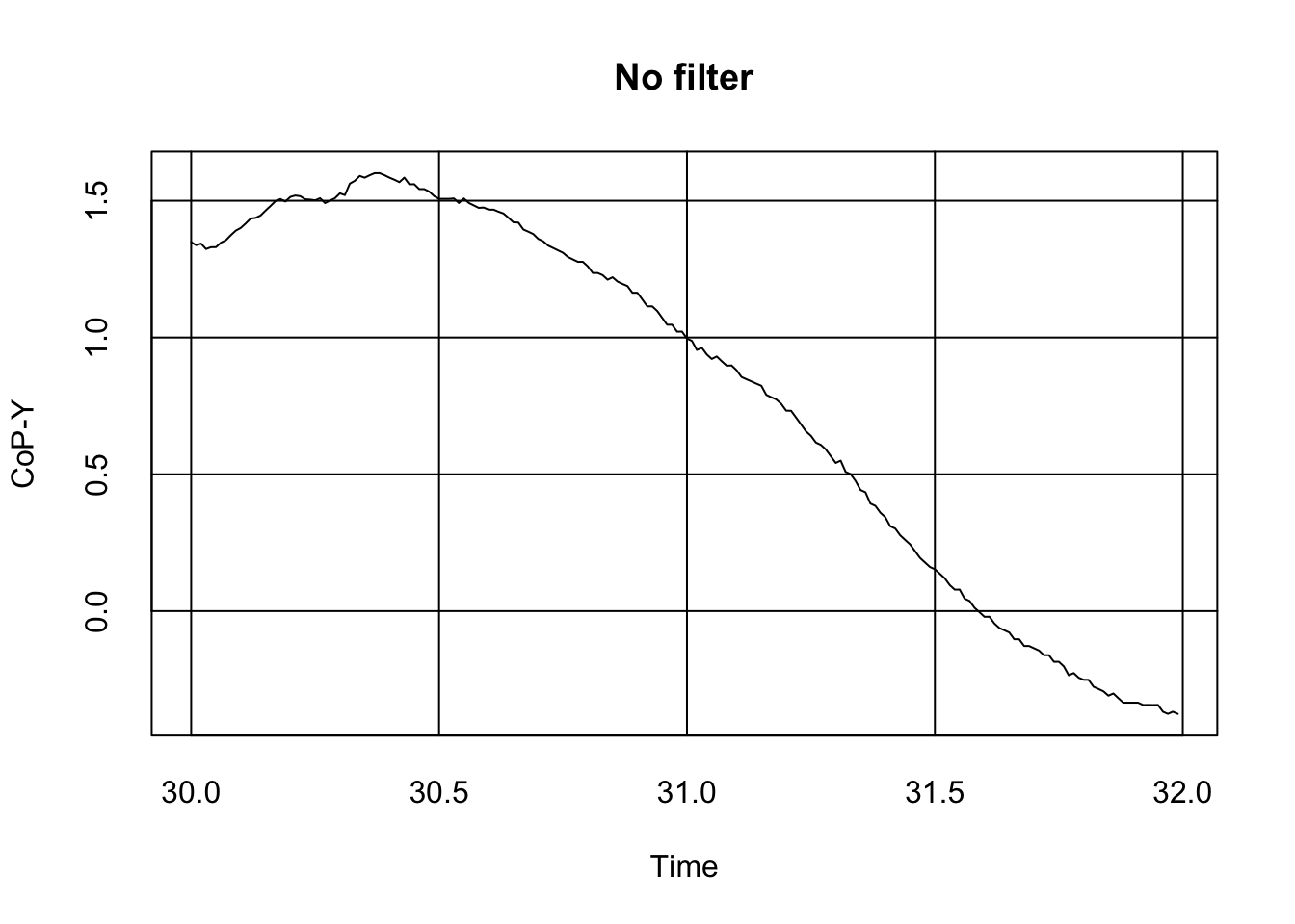

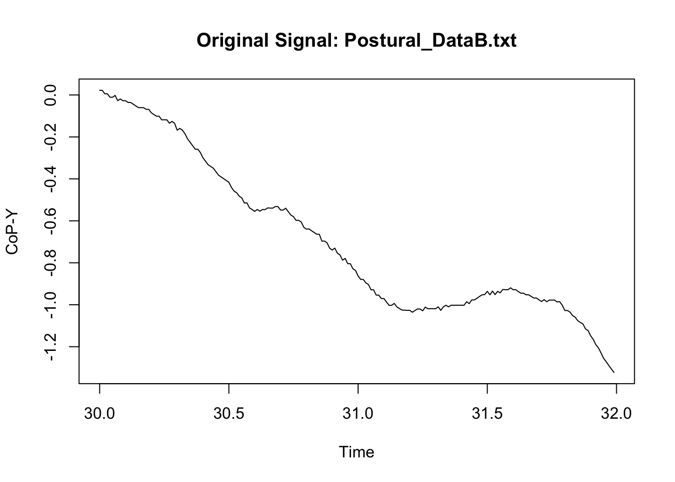
plot(x = subset(Data, Data$file_name == "Postural_DataB.txt" & Data$Time > 30 & Data$Time < 32)$Time, 
     y = subset(Data, Data$file_name == "Postural_DataB.txt" & Data$Time > 30 & Data$Time < 32)$CoP_Y, type ="l", tck = 1, main = "No filter", xlab = "Time", ylab = "CoP-Y")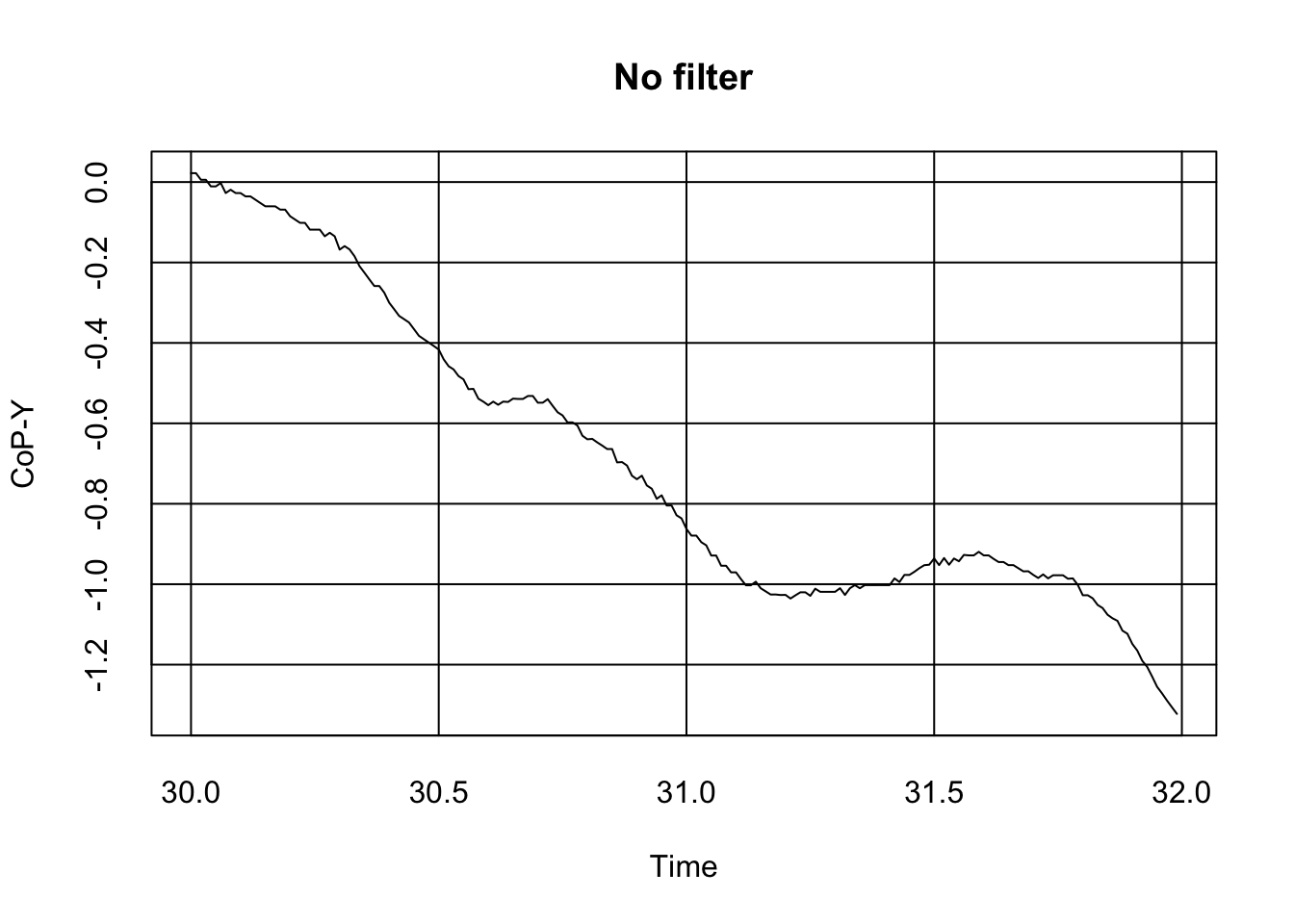

plot(x = subset(Data, Data$file_name == "Postural_DataA.txt" & Data$Time > 30 & Data$Time < 32)$Time, 
     y = subset(Data, Data$file_name == "Postural_DataA.txt" & Data$Time > 30 & Data$Time < 32)$CoP_Y, type ="l", tck = 1, main = "No filter", xlab = "Time", ylab = "CoP-Y")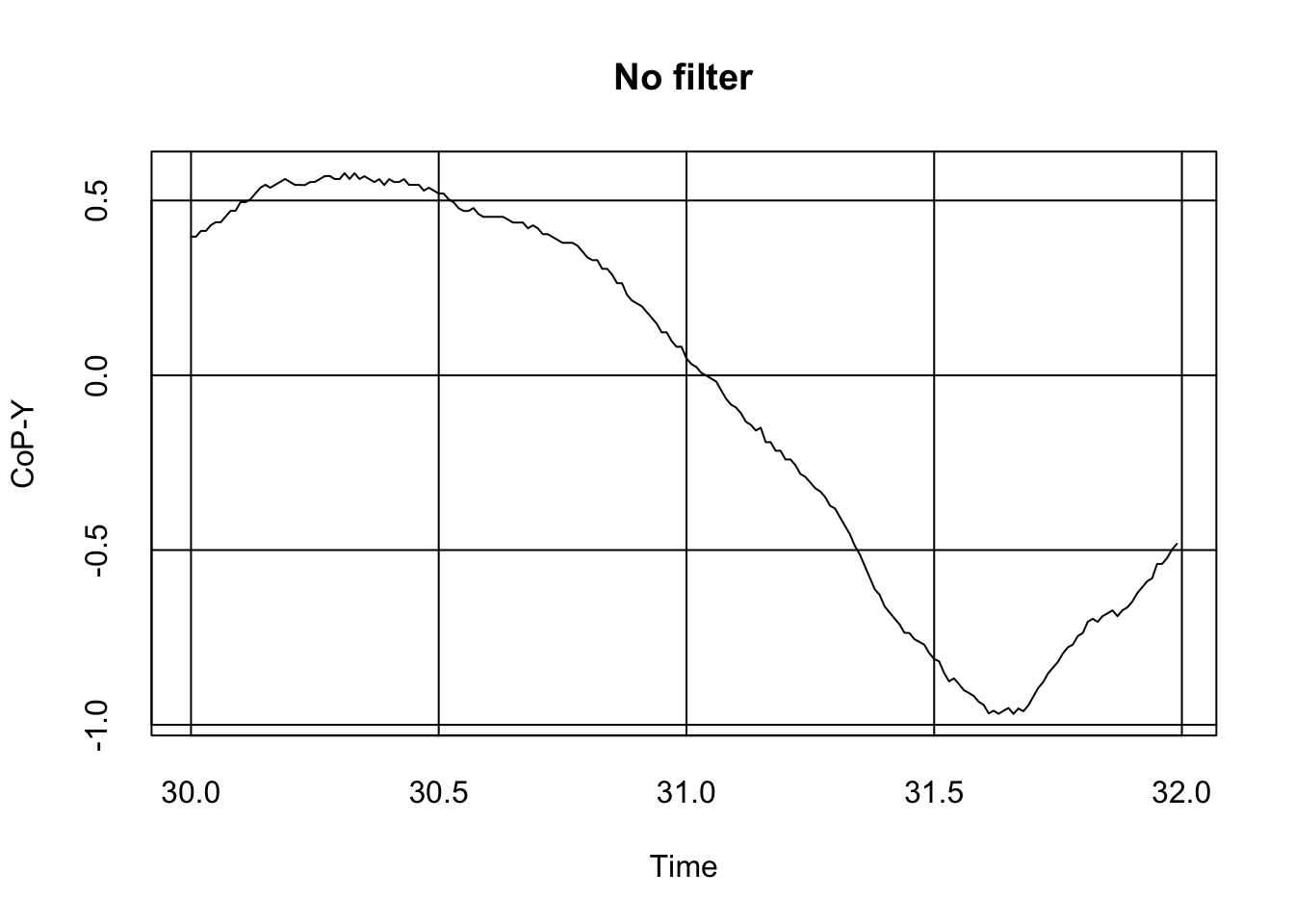

plot(x = subset(Data, Data$file_name == "Postural_DataD.txt" & Data$Time > 30 & Data$Time < 32)$Time, 
     y = subset(Data, Data$file_name == "Postural_DataD.txt" & Data$Time > 30 & Data$Time < 32)$CoP_Y, type ="l", tck = 1, main = "No filter", xlab = "Time", ylab = "CoP-Y")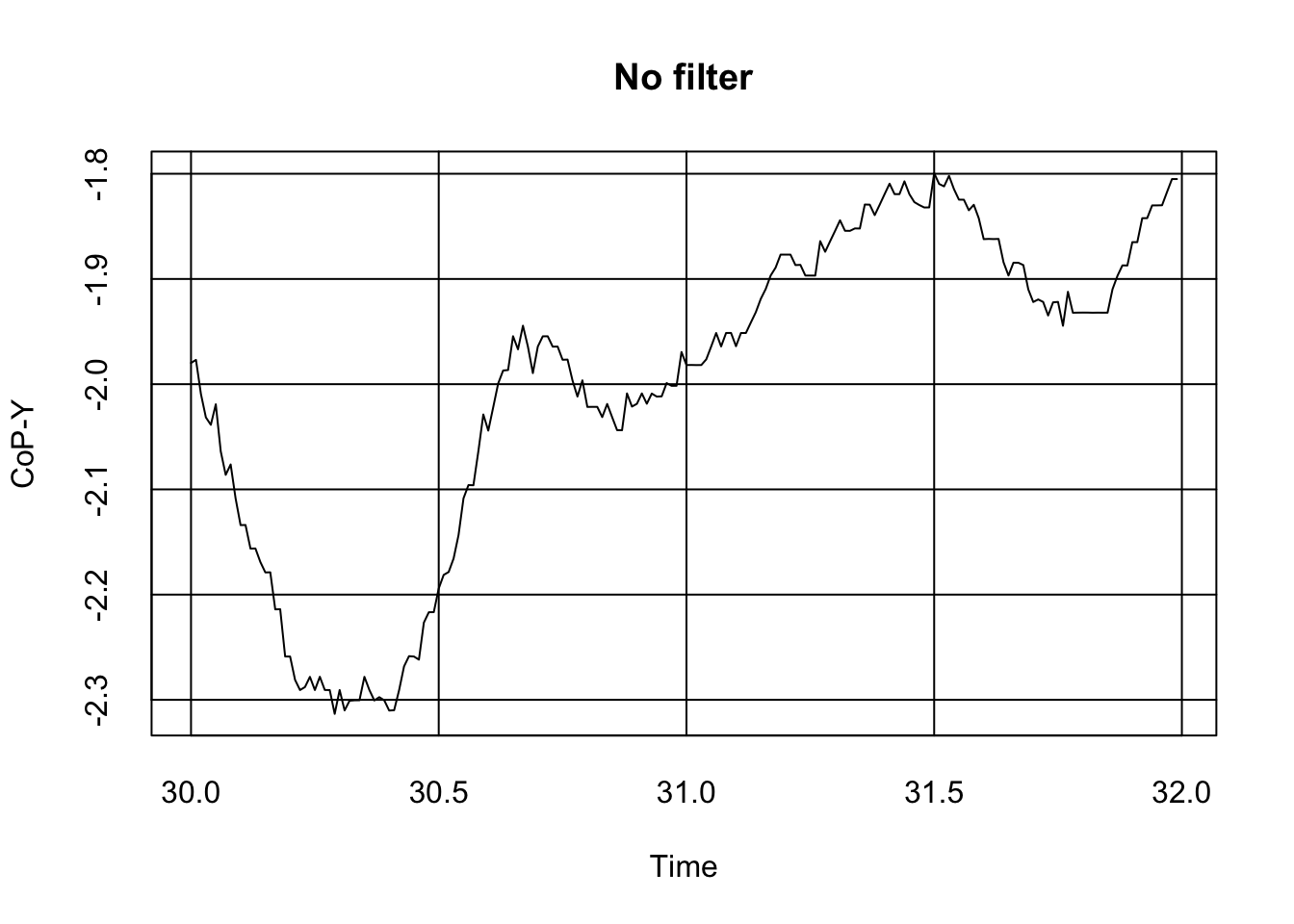

plot(x = subset(Data, Data$file_name == "Postural_DataE.txt" & Data$Time > 30 & Data$Time < 32)$Time, 
     y = subset(Data, Data$file_name == "Postural_DataE.txt" & Data$Time > 30 & Data$Time < 32)$CoP_Y, type ="l", tck = 1, main = "No filter", xlab = "Time", ylab = "CoP-Y")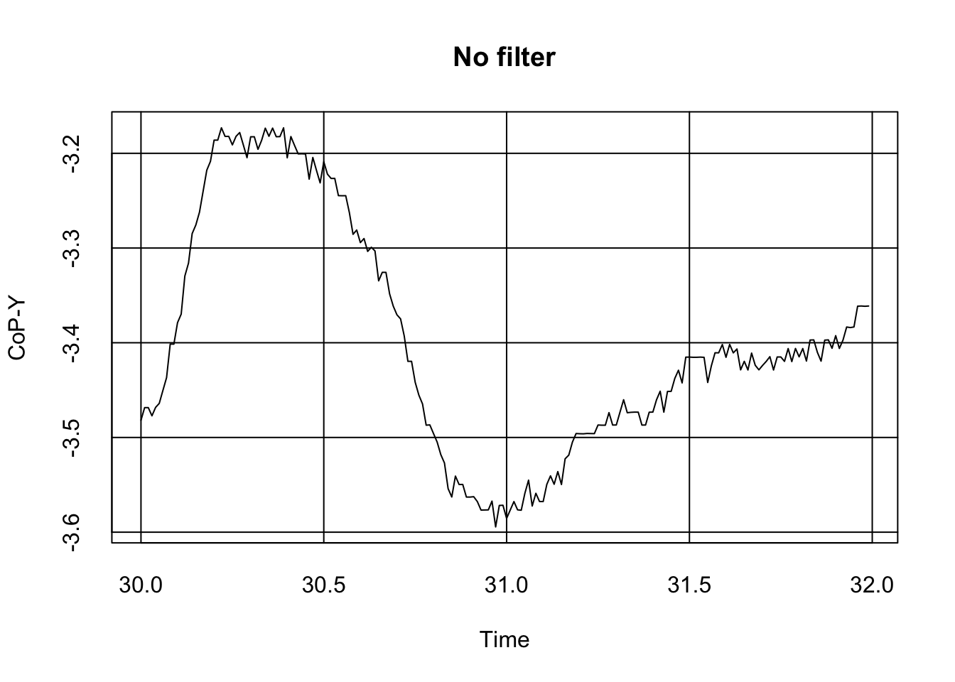

As we can see, the signal is a bit messy, including tiny spikes that might make the reading awkward. Although some authors shrug this issue away (after all, error is possibly randomly distributed around the true signal value, and as such, in the long run, it should not matter much), some authors might want to get the best signal possible by applying filters.

2.0.1 A short digression on signals

The author of this package being quite naive regarding signal filters (interested readers are re-directed to the signal package), it can be noted that – drawing on the literature on approach and avoidance of (un)pleasant stimuli, some types of filters are more popular than others (see Table X). In particular the most used type of filters would be: No filter at all, a 2nd order low-pass Butterworth filter with a cut-off frequency of 5Hz, and then a 2nd order low-pass Butterworth filter with a cut-off frequency of 10Hz.

Table 2.1: Cut-Off Frequency usage in the literature

Cut-off Frequency used	Number of papers
10Hz	5
15Hz	1
20Hz	1
5Hz	8
8Hz	1
No filter used	25
Not enough information	2
Other	1

Table 2.1: Filter’s order usage in the literature

Order of the filter used	Number of papers
2nd Order	10
3rd Order	1
N/A	26
Unknown	7

Regarding high vs low-pass; it appears all filters either mention explicitly using a low-pass filter, or do not report which type of filter they used.

Note: other types of filter where 5-points moving average (n = 1).

The author of the current package does not endorse any stance regarding whether or not it is advisable to transform signal through a filter. However, should the reader prefer data filtering, it would be recommended to register data processing beforehand to avoid any excessive flexibility in how data is handled. After all, like R. Feynman said “Rule number 1 is to not fool yourself, and you are the easiest person to fool.”

Nevertheless, it is worth mentionning that most authors recommend plotting the signal after filtering to make sure that the type of filter you used did not result in weird signals. It happens. We also recommend to plot the transformed signal and maybe try which one provides the best type of signal visually. Because this process is difficult to register, readers willing to filter their signal data should strive for a transparent approach. Different filters would be tested and sample results of the new signals would be reported (for instance, in supplementary online material or an OSF webpage) for reviewers to assess. In the end, choice of a filter requires a justification.

For the sake of brevity, or - let’s say - to encourage a standardisation of the practices, the package does not offer any other filter than the widely used Butterworth filter.

2.0.2 Butterworth_it: apply a custom Butterworth filter to your signal

Butterworth filter is by far the most used type of filter. It is a wrapper of the filtfilt command of the signal package. To use it, you need to specify the column(s) you want to filter, indicate the order you want to use, the cut-off frequency for the filter, and whether you would like a high or low-pass filter to be applied..

D’Api and De Reinette want to use a 2nd order Butterworth filter with a cut-off frequency of 5Hz. They based their choice on the popularity of this specific filter (see Monéger et al., 2024 [preprint]).

Note: the filter is used on the raw data, before any synthesis is done. It can be applied to the moments and forces (used to compute CoP), or on the CoP itself – this does not produce much difference from what I have tested. Because the filter is applied on raw data, the computation might take some time for large datasets. Let’s assume we are doing ‘slow science’ here.

Data<-Merge_PosData("~/Desktop/BalanceMate/inst/extdata/", SampleRate = 100, SessionDuration = 100)
filtered_data <- Butterworth_it(
  Data = Data,
  cutoff_freq = 5,
  filter_order = 2,
  sampling_rate = 100,
  type = "low",
  Colname = c("CoP_X", "CoP_Y")
)

The resulting data file contains now one column with the raw untransformed signal and one column with the filtered signal.

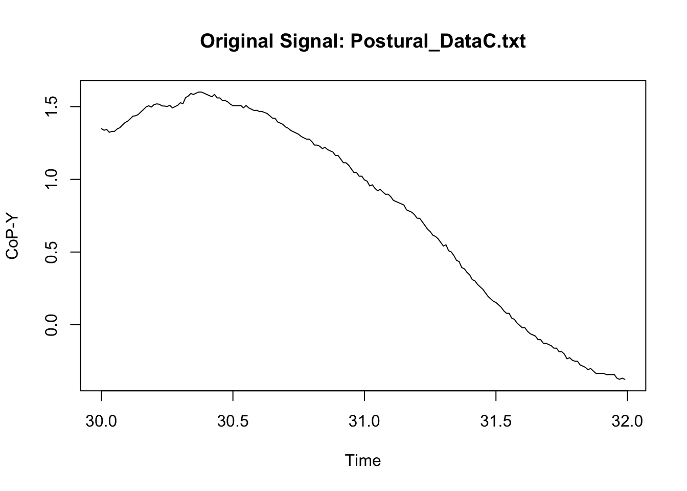
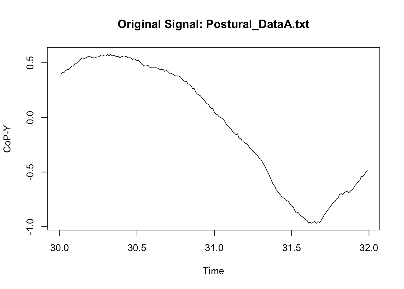
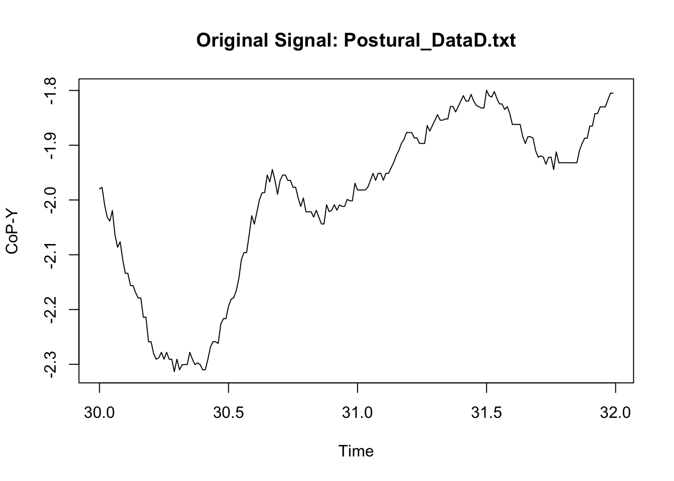
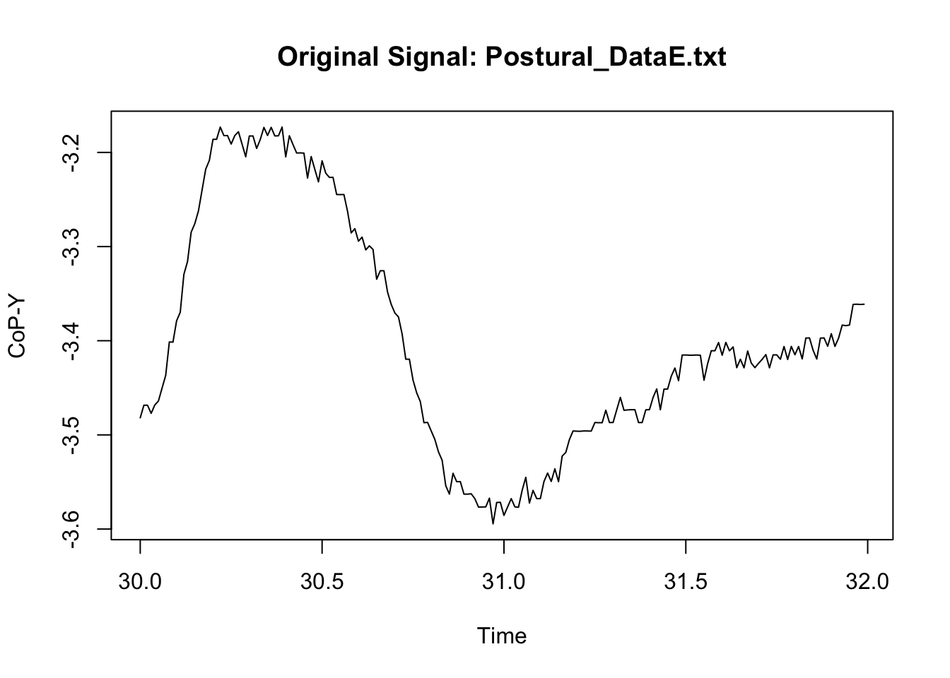
We can now compare the original signal to the filtered signal to assess whether the filter did not result in some weird signal. Because we have a lot of data, I only illustrate here what happened in a specific sample of measures in one participant (I however do recommend that users try multiple samples including the beginning and the end of specific trial; see for instance: https://stackoverflow.com/questions/67847747/butterworth-filter-results-in-extreme-outliers-at-start-of-the-signal).

# File names
file_names <- c("Postural_DataC.txt", "Postural_DataB.txt", "Postural_DataA.txt", "Postural_DataD.txt", "Postural_DataE.txt")

# Loop through file names to generate plots side by side
for (file in file_names) {
  # Original signal plot
  plot(
    x = subset(filtered_data, filtered_data$file_name == file & filtered_data$Time > 30 & filtered_data$Time < 32)$Time,
    y = subset(filtered_data, filtered_data$file_name == file & filtered_data$Time > 30 & filtered_data$Time < 32)$CoP_Y,
    type = "l",
    main = paste("Original Signal:", file),
    xlab = "Time",
    ylab = "CoP-Y"
  )
  
  # Filtered signal plot
  plot(
    x = subset(filtered_data, filtered_data$file_name == file & filtered_data$Time > 30 & filtered_data$Time < 32)$Time,
    y = subset(filtered_data, filtered_data$file_name == file & filtered_data$Time > 30 & filtered_data$Time < 32)$CoP_Y_filtered,
    type = "l",
    main = paste("Filtered Signal:", file),
    xlab = "Time",
    ylab = "CoP-Y"
  )
}

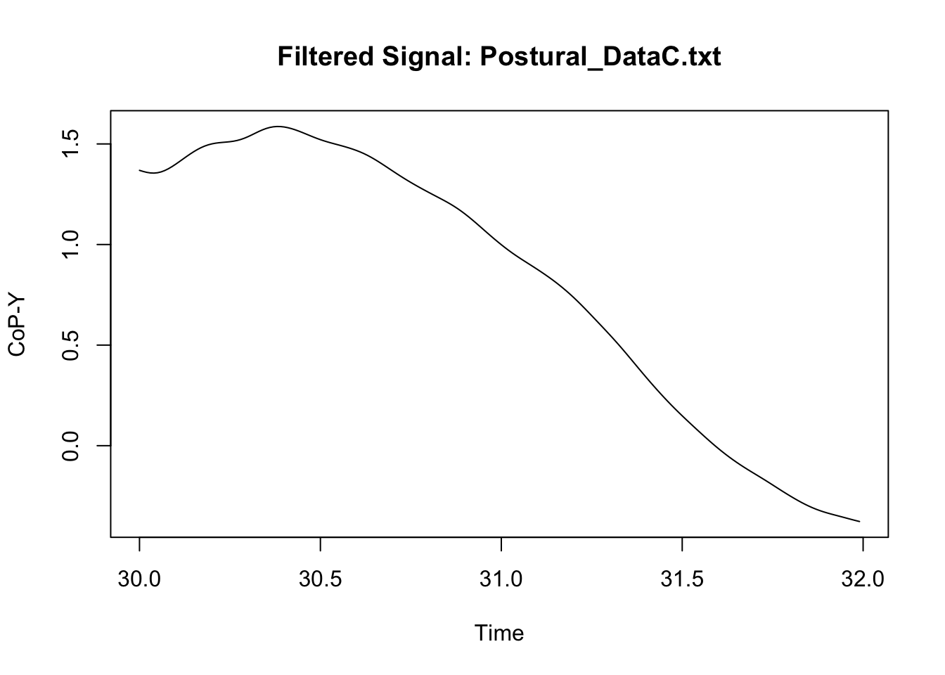
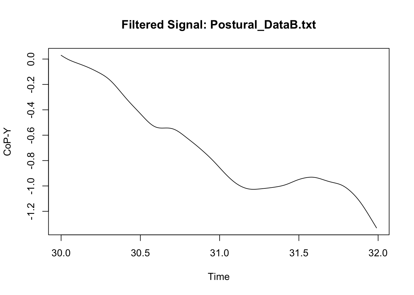
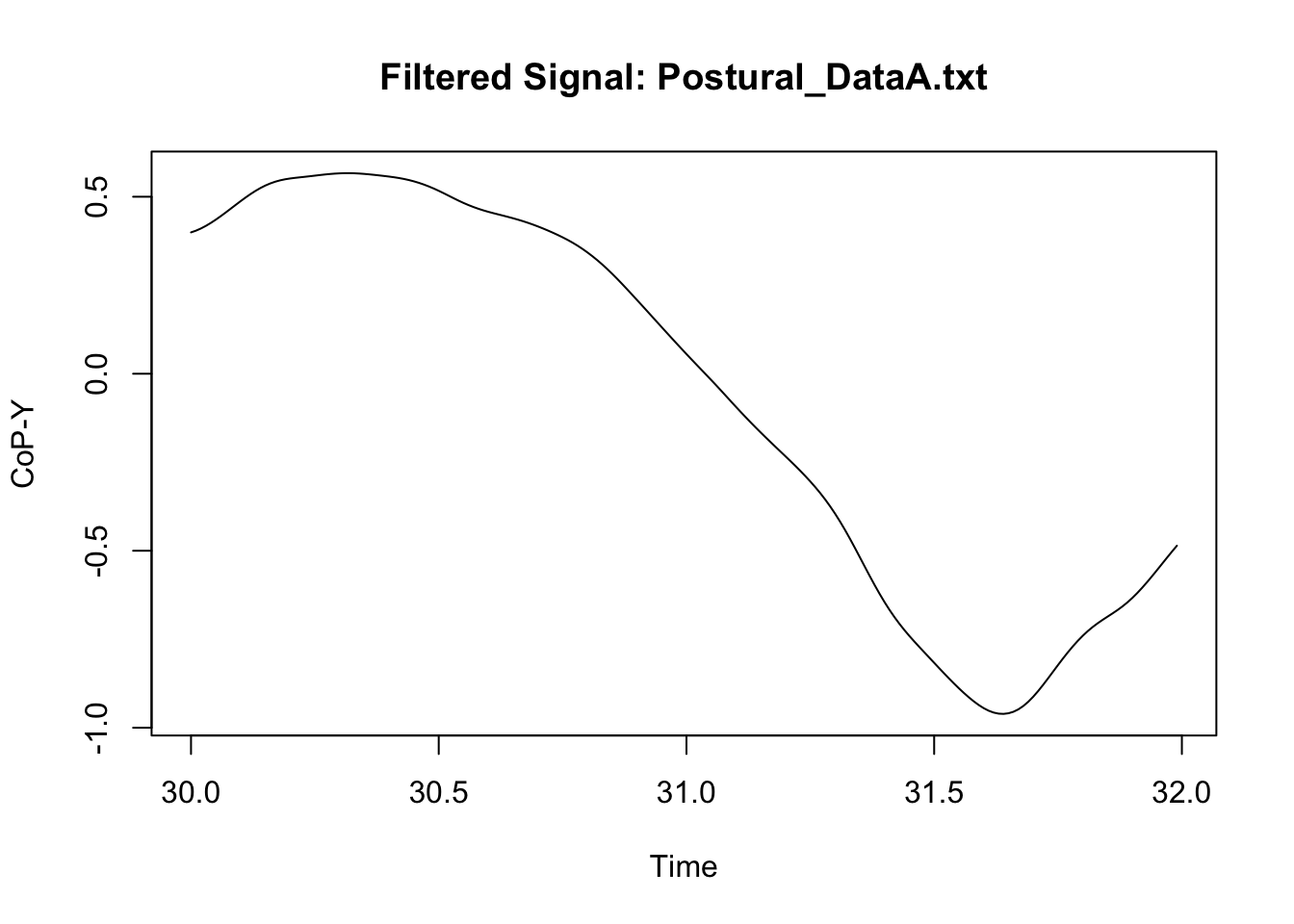
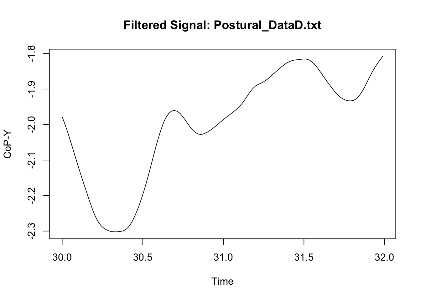
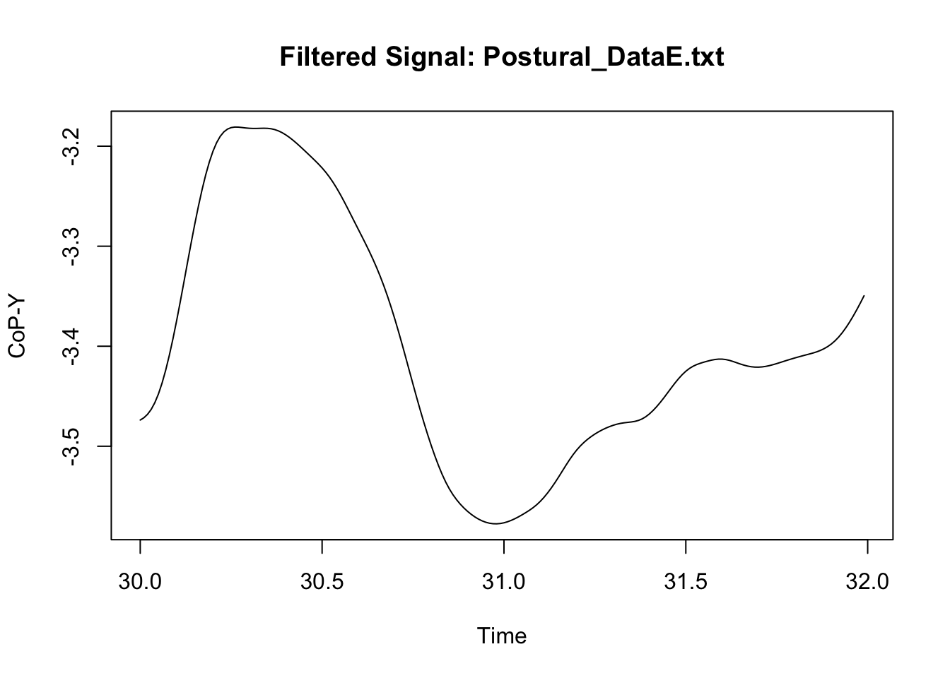
This looks neat. We can then synthetise the data at a specific time-bin level if we wish to, or manage the new signal in any possible way (see Chapter 1: Managing).

Once we have our data ready, we can jump into the most exciting part of our journey: processing the postural data.