R session Environment

Toggle details regarding my R environment: packages and machine

Loading packages:

if(!require("dplyr")) install.packages("dplyr")
if(!require("tidyr")) install.packages("tidyr")
if(!require("stringr")) install.packages("stringr")
if(!require("ggplot2")) install.packages("ggplot2")
if(!require("emmeans")) install.packages("emmeans")
if(!require("data.table")) install.packages("data.table")
if(!require("PerformanceAnalytics")) install.packages("PerformanceAnalytics")
if(!require("interactions")) install.packages("interactions")
if(!require("car")) install.packages("car")
if(!require("effectsize")) install.packages("effectsize")
if(!require("RColorBrewer")) install.packages("RColorBrewer")
if(!require("report")) install.packages("report")
if(!require("robustbase")) install.packages("robustbase") # For Minimum Covariance distance
if(!require("knitr")) install.packages("knitr")
if(!require("gt")) install.packages("gt")
if(!require("lavaan")) install.packages("lavaan")
if(!require("ppcor")) install.packages("ppcor") # For partial correlations
if(!require("sjPlot")) install.packages("sjPlot")
if(!require("MASS")) install.packages("MASS")
if(!require("Matrix")) install.packages("Matrix")
if(!require("ggrepel")) install.packages("ggrepel")
if(!require("corrplot")) install.packages("corrplot")
if(!require("plotly")) install.packages("plotly") # Interactive plots <3
if(!require("performance")) install.packages("performance") 
if(!require("partR2")) install.packages("partR2") 
if(!require("multcomp")) install.packages("multcomp") 
if(!require("parameters")) install.packages("parameters") 
if(!require("lme4")) install.packages("lme4") 
if(!require("lmerTest")) install.packages("lmerTest") 
if(!require("MuMIn")) install.packages("MuMIn") 
if(!require("gridExtra")) install.packages("gridExtra") # Plot layout
if(!require("purrr")) install.packages("purrr") # Really cool 3D scatterplots
if(!require("olsrr")) install.packages("olsrr") # 
if(!require("modelsummary")) install.packages("modelsummary") #

Session info:

sessionInfo()

## R version 4.5.1 (2025-06-13)
## Platform: aarch64-apple-darwin20
## Running under: macOS Sonoma 14.7.1
## 
## Matrix products: default
## BLAS:   /Library/Frameworks/R.framework/Versions/4.5-arm64/Resources/lib/libRblas.0.dylib 
## LAPACK: /Library/Frameworks/R.framework/Versions/4.5-arm64/Resources/lib/libRlapack.dylib;  LAPACK version 3.12.1
## 
## locale:
## [1] en_US.UTF-8/en_US.UTF-8/en_US.UTF-8/C/en_US.UTF-8/en_US.UTF-8
## 
## time zone: Europe/London
## tzcode source: internal
## 
## attached base packages:
## [1] stats     graphics  grDevices utils     datasets  methods   base     
## 
## other attached packages:
##  [1] modelsummary_2.5.0         olsrr_0.6.1               
##  [3] purrr_1.1.0                gridExtra_2.3             
##  [5] MuMIn_1.48.11              lmerTest_3.1-3            
##  [7] lme4_1.1-37                parameters_0.28.2         
##  [9] multcomp_1.4-28            TH.data_1.1-4             
## [11] survival_3.8-3             mvtnorm_1.3-3             
## [13] partR2_0.9.2               performance_0.15.1        
## [15] plotly_4.11.0              corrplot_0.95             
## [17] ggrepel_0.9.6              Matrix_1.7-3              
## [19] sjPlot_2.9.0               ppcor_1.1                 
## [21] MASS_7.3-65                lavaan_0.6-20             
## [23] gt_1.1.0                   knitr_1.50                
## [25] robustbase_0.99-6          report_0.6.1              
## [27] RColorBrewer_1.1-3         effectsize_1.0.1          
## [29] car_3.1-3                  carData_3.0-5             
## [31] interactions_1.2.0         PerformanceAnalytics_2.0.8
## [33] xts_0.14.1                 zoo_1.8-14                
## [35] data.table_1.17.8          emmeans_1.11.2-8          
## [37] ggplot2_4.0.0              stringr_1.5.2             
## [39] tidyr_1.3.1                dplyr_1.1.4               
## 
## loaded via a namespace (and not attached):
##  [1] Rdpack_2.6.4        mnormt_2.1.1        sandwich_3.1-1     
##  [4] rlang_1.1.6         magrittr_2.0.4      furrr_0.3.1        
##  [7] compiler_4.5.1      vctrs_0.6.5         quadprog_1.5-8     
## [10] pkgconfig_2.0.3     fastmap_1.2.0       backports_1.5.0    
## [13] pbivnorm_0.6.0      pander_0.6.6        rmarkdown_2.29     
## [16] nloptr_2.2.1        xfun_0.53           cachem_1.1.0       
## [19] jsonlite_2.0.0      goftest_1.2-3       broom_1.0.10       
## [22] parallel_4.5.1      R6_2.6.1            tables_0.9.31      
## [25] bslib_0.9.0         stringi_1.8.7       parallelly_1.45.1  
## [28] boot_1.3-31         numDeriv_2016.8-1.1 jquerylib_0.1.4    
## [31] estimability_1.5.1  Rcpp_1.1.0          splines_4.5.1      
## [34] tidyselect_1.2.1    rstudioapi_0.17.1   abind_1.4-8        
## [37] yaml_2.3.10         codetools_0.2-20    listenv_0.9.1      
## [40] lattice_0.22-7      tibble_3.3.0        withr_3.0.2        
## [43] bayestestR_0.17.0   S7_0.2.0            coda_0.19-4.1      
## [46] evaluate_1.0.5      future_1.67.0       xml2_1.4.0         
## [49] jtools_2.3.0        pillar_1.11.1       nortest_1.0-4      
## [52] stats4_4.5.1        reformulas_0.4.1    insight_1.4.2      
## [55] generics_0.1.4      scales_1.4.0        minqa_1.2.8        
## [58] globals_0.18.0      xtable_1.8-4        glue_1.8.0         
## [61] lazyeval_0.2.2      tools_4.5.1         forcats_1.0.0      
## [64] fs_1.6.6            grid_4.5.1          rbibutils_2.3      
## [67] datawizard_1.2.0    nlme_3.1-168        Formula_1.2-5      
## [70] cli_3.6.5           viridisLite_0.4.2   gtable_0.3.6       
## [73] DEoptimR_1.1-4      broom.mixed_0.2.9.6 sass_0.4.10        
## [76] digest_0.6.37       htmlwidgets_1.6.4   farver_2.1.2       
## [79] htmltools_0.5.8.1   lifecycle_1.0.4     httr_1.4.7

What we know of occupational heroism

Some occupations are more likely than others to be perceived as being heroic. We have consistently shown that these occupations were qualified by high helpfulness perception and high exposure do danger perception. However, a central part of our research project is to identify the consequences (both positive and negative) of having one’s occupation perceived as heroic. We propose that occupational heroism can predict:

H1: Higher gratitude toward workers
H2: Reduced criticism acceptability
H3: Decreased support for demands from the workers
H4: Decreased perception of victim-related aspects (e.g., suffering, vulnerability)
H5: Increased impunity and motivation to de-regulate the occupation

While pilot testing the main questionnaire that was used in this study, we found mixed support for our hypotheses. Our pilot test used police officers as a target occupation and, in a sample of 440 representative UK residents, we found evidence for H1, H2, and H5; but not for H3 and H4. In fact, we observed that heroism predicted increased victim-perception and increased support for workers’ demands. These findings held even after accounting for attitude toward police officers.

We now test our main hypotheses in a larger sample of occupations: Nurses, Psychiatrists, Underwater welders, Journalists, Soldiers an Firefighters.

In particular, we had 3 typically heroic occupations (Nurses, Soldiers, Firefighters); and 3 Non-heroic occupations (Psychiatrists, Journalists, and Underwater Welders).

The study was registered online: https://osf.io/e3mhs

The study gained ethical approval from the University of Kent: Ethics ID 2025175820653410122

Materials and Data is available online: https://osf.io/6gpz7/

In addition, a shiny app is available to interactively explore the main results of this study: https://jeanmoneger.shinyapps.io/Explorer_C1_Septembre/

cat(’

’)

#inline-toc { border: 1px solid #ddd; border-radius: 8px; padding: 0.75rem; margin: 1rem 0; }

Data Wrangling

From the chaotic Qualtrics export, we organise a long format data frame with one row per participant, with their condition (target occupation) neatly organised in one columns. Details of the data wrangling are given below.

Toggle details of the data wrangling procedure

Adapt the path of the data file to your local path. We recommend putting all the files in a single folder containing the rmd file.

DF <- read.csv("Data_Correlational_C1.csv", comment.char="#")
DF <- subset(DF, DF$age != "")
Demographics <- DF[-c(1:2), c(269:278)]
DF <- DF[-c(1:2), c(23, 25:44, 49:268, 281)]

prolOK <- read.csv("Prolific_Export_C1.csv")

AwaitR<- subset(prolOK, prolOK$Status == "APPROVED")

DF <- subset(DF, DF$prolID != setdiff(DF$prolID, AwaitR$Participant.id))


Journ <- subset(DF, DF$Cond == "Journalist")
Journ <- Journ[, colSums(!is.na(Journ) & Journ != "") > 0 | grepl("SpecCritJ", names(Journ)), drop = FALSE]


Fire <- subset(DF, DF$Cond == "Firefighter")
Fire <- Fire[, colSums(!is.na(Fire) & Fire != "") > 0 | grepl("SpecCritF", names(Fire)), drop = FALSE]

Nurs <- subset(DF, DF$Cond == "Nurse")
Nurs <- Nurs[, colSums(!is.na(Nurs) & Nurs != "") > 0 | grepl("SpecCritN", names(Nurs)), drop = FALSE]

Psych <- subset(DF, DF$Cond == "Psych")
Psych <- Psych[, colSums(!is.na(Psych) & Psych != "") > 0 | grepl("SpecCritP", names(Psych)), drop = FALSE]

Soldier <- subset(DF, DF$Cond == "Soldier")
Soldier <- Soldier[, colSums(!is.na(Soldier) & Soldier != "") > 0 | grepl("SpecCritS", names(Soldier)), drop = FALSE]

Weld <- subset(DF, DF$Cond == "Weld")
Weld <- Weld[, colSums(!is.na(Weld) & Weld != "") > 0 | grepl("SpecCritW", names(Weld)), drop = FALSE]


# 1) Use Weld as the "template" for column names
template_names <- names(Weld)  # 47 names

# 2) Helper that renames a data frame by POSITION to match Weld
rename_like_weld <- function(df, template = template_names) {
  # Sanity checks to avoid silent disasters
  if (ncol(df) != length(template)) {
    stop("Column count mismatch: this df has ", ncol(df),
         " columns but template has ", length(template), ".")
  }
  # Copy names by position
  names(df) <- template
  df
}

# 3) Put all your data frames into a named list
dfs <- list(
  Weld    = Weld,
  Journ   = Journ,
  Nurs    = Nurs,
  Psych   = Psych,
  Soldier = Soldier,
  Fire    = Fire
)

# 4) Harmonise names, then stack vertically with a source column
stacked <- dfs %>%
  purrr::map(rename_like_weld) %>%          # harmonise titles to Weld's names
  bind_rows(.id = "dataset")         # adds the dataset name as the first column

# Result: 48 columns total (1 "dataset" + 47 harmonised vars)
# and nrow(stacked) == sum(nrow(.) for each df)



#------------------------------------------------------------
# 0) Small helpers
#------------------------------------------------------------

# Replace "" and pure whitespace with NA
na_empty <- function(x) {
  x <- if (is.character(x)) str_trim(x) else x
  ifelse(is.character(x) & x == "", NA, x)
}

# Map character -> numeric using a named vector `key`.
# Unknown labels become NA (so you’ll notice and can fix the key).
map_to_num <- function(x, key) {
  x <- na_empty(x)
  # exact match after trimming
  out <- unname(key[ match(x, names(key)) ])
  # if x is already numeric-like (e.g., "5"), keep it
  suppressWarnings({
    out_numlike <- as.numeric(x)
  })
  out[is.na(out) & !is.na(out_numlike)] <- out_numlike[is.na(out) & !is.na(out_numlike)]
  as.numeric(out)
}

# Pull the first integer in a string like "7 - Strongly agree" -> 7
first_int <- function(x) {
  x <- na_empty(x)
  as.numeric(str_extract(x, "\\d+"))
}

# Checkbox columns: any non-empty text -> 1, blank/NA -> 0
checkbox01 <- function(x) as.numeric(!is.na(na_empty(x)))


#------------------------------------------------------------
# 1) Define your scale keys (edit here if wording differs)
#------------------------------------------------------------

agree7 <- c(
  "Strongly disagree"             = 1,
  "Moderately disagree"           = 2,
  "Slightly disagree"             = 3,
  "Neither disagree, nor agree"   = 4,
  "Slightly agree"                = 5,
  "Moderately agree"              = 6,
  "Strongly agree"                = 7
)

likely7 <- c(
  "Very unlikely"                 = 1,
  "Quite unlikely"                = 2,
  "Slightly unlikely"             = 3,
  "Neither likely, nor unlikely"  = 4,
  "Slightly likely"               = 5,
  "Quite likely"                  = 6,
  "Very likely"                   = 7
)

# Frequency (seen in GenSuppDemWeld_*): includes "Always" at the top end
freq7 <- c(
  "Never"            = 1,
  "Very Rarely"      = 2,
  "Rarely"           = 3,  
  "Occasionally"     = 4,
  "Frequently"       = 5,
  "Very frequently"  = 6,
  "Always"           = 7
)

# Intensity (seen in GenVictimWeld_*): ordered least -> most
intensity7 <- c(
  "Not at all"   = 1,
  "Very little"  = 2,
  "A little"     = 3,
  "Somewhat"     = 4,
  "Quite a bit"  = 5,
  "A lot"        = 6,
  "Very much"    = 7 #!!!!!

)

# Valence (Q239). Your data shows: Very/Quite negative, Somewhat/Quite/Very positive.
# Map to 1..5 (negative -> positive). If you have "Neither", add it as 3.
valence5 <- c(
  "Very negative"      = 1,
  "Quite negative"            = 2, 
  "Somewhat negative"     = 3, #!!!!!!
  "Neutral"  = 4,
  "Somewhat positive"     = 5,  
  "Quite positive"      = 6,
  "Very positive" = 7
)

# Gratitude single item (GenGratWeld) appears to use intensity-style words
grat7 <- intensity7


#------------------------------------------------------------
# 2) Identify column groups by name (using your Weld names)
#    We only target cols 2:41, but naming groups is clearer & safer.
#------------------------------------------------------------

agree_cols <- c(
  # Crit accept (general)
  "GenCritW_1","GenCritW_2","GenCritW_3",
  # Specific victims/villains attitudes (agree-type)
  "SpecSuppW_1","SpecSuppW_2","SpecSuppW_3",
  "SpecVictimW_1","SpecVictimW_2","SpecVictimW_3",
  "GenImpW_1","GenImpW_2","GenImpW_3","GenImpW_4",
  "SpecImpW_1","SpecImpW_2","SpecImpW_3","SpecImpW_4"
)

likely_cols <- c("SpecGratW_1","SpecGratW_2","SpecGratW_3")

freq_cols <- c("GenSuppW_1","GenSuppW_2")

intensity_cols <- c("GenVictW_1","GenVictW_2","GenVictW_3","GeneralGratW")

# Checkbox blocks (present/blank -> 1/0)
checkbox_cols <- c(
  "SpecCritW1_1","SpecCritW1_2","SpecCritW1_3","SpecCritW1_9","SpecCritW1_4",
  "SpecCritW2_1","SpecCritW2_2","SpecCritW2_3","SpecCritW2_9","SpecCritW2_4"
)

# Hybrid numeric-label items
hybrid_num_cols <- c("HW_1","DangerHelpW_1","DangerHelpW_2")

# Valence item
valence_cols <- c("AttW")


#------------------------------------------------------------
# 3) Apply mappings to your stacked data (called `stacked`)
#    We leave identifying/meta columns alone: dataset, prolID, gender*, age, Q52, Attentive, Cond
#------------------------------------------------------------

stacked_num <- stacked %>%
  mutate(
    # scales
    across(all_of(agree_cols),    ~ map_to_num(.x, agree7)),
    across(all_of(likely_cols),   ~ map_to_num(.x, likely7)),
    across(all_of(freq_cols),     ~ map_to_num(.x, freq7)),
    across(all_of(intensity_cols),~ map_to_num(.x, intensity7)),
    across(all_of(valence_cols),  ~ map_to_num(.x, valence5)),

    # checkbox-style -> 0/1
    across(all_of(checkbox_cols), checkbox01),

    # hybrid numerics (e.g., "7 - Strongly agree" or just "5")
    across(all_of(hybrid_num_cols), first_int),

    )


#colnames(stacked_num)

# Check results by uncommenting lines below:
#compare_freqs <- function(char_df, num_df, col) {
#    cat("\n\n###", col, "###\n")
#    
#    char_counts <- as.data.frame(table(char_df[[col]]), stringsAsFactors = FALSE)
#    num_counts  <- as.data.frame(table(num_df[[col]]), stringsAsFactors = FALSE)
#    
#    names(char_counts) <- c("label", "char_n")
#    names(num_counts)  <- c("num_value", "num_n")
#    
#    # Make sure numeric column is actually numeric for sorting
#    suppressWarnings(num_counts$num_value <- as.numeric(as.character(num_counts$num_value)))
#    num_counts <- num_counts[order(num_counts$num_value), ]
#    
#    # Match by frequency
#    matched_labels <- character(nrow(num_counts))
#    matched_char_n <- integer(nrow(num_counts))
#    errors <- character(0)
#    
#    for (i in seq_len(nrow(num_counts))) {
#        n <- num_counts$num_n[i]
#        match_rows <- which(char_counts$char_n == n)
#        
#        if (length(match_rows) == 1) {
#            matched_labels[i] <- char_counts$label[match_rows]
#            matched_char_n[i] <- char_counts$char_n[match_rows]
#        } else if (length(match_rows) > 1) {
#            # ambiguous match → keep first
#            matched_labels[i] <- char_counts$label[match_rows[1]]
#            matched_char_n[i] <- char_counts$char_n[match_rows[1]]
#        } else {
#            # no match → flag error
#            matched_labels[i] <- NA
#            matched_char_n[i] <- NA
#            errors <- c(errors, paste0("No matching label for numeric value ", num_counts$num_value[i],
#                                       " (n=", n, ")"))
#        }
#    }
#    
#    comparison <- data.frame(
#        num_value = num_counts$num_value,
#        num_n = num_counts$num_n,
#        label = matched_labels,
#        char_n = matched_char_n,
#        stringsAsFactors = FALSE
#    )
#    
#    print(comparison, row.names = FALSE)
#    
#    if (length(errors) > 0) {
#        cat("⚠️  Errors:\n", paste0(" - ", errors, collapse = "\n"), "\n")
#    }
#}
#
## Columns to check
#cols_to_check <- setdiff(names(stacked), c("dataset", "Q90", "Attentive", "Cond"))
#
## Run it
#for (col in cols_to_check) {
#    compare_freqs(stacked, stacked_num, col)
#}


# Remove ATTENTION CHECKS
stacked_num <- stacked_num[, -c(21, 31, 33)]




# Severity mapping: column suffix -> numeric severity
severity_map <- c("1" = 1, "2" = 2, "3" = 3, "9" = 4, "4" = 5)

# Helper: collapse one multi-response item (five 0/1 columns) into a single 1..5 severity
most_severe <- function(data, stem, map = severity_map) {
  # Build the expected column names for this stem
  suf  <- names(map)                           # c("1","2","3","9","4")
  cols <- paste0(stem, "_", suf)

  # Safety checks: are all expected columns present?
  missing <- setdiff(cols, names(data))
  if (length(missing)) {
    stop("Missing columns for '", stem, "': ", paste(missing, collapse = ", "))
  }

  # Grab the indicators as a numeric matrix (0/1/NA)
  M <- as.matrix(data[cols])

  # Treat 0 as "not selected" -> NA, so they don't affect the max
  M[M == 0] <- NA

  # Weight each column by its severity value (1..5) so max() = most severe chosen
  sev <- as.numeric(map)
  W   <- sweep(M, 2, sev, `*`)   # column j multiplied by sev[j]

  # Row-wise max ignoring NAs; if all NA -> NA
  out <- apply(W, 1, function(x) {
    m <- suppressWarnings(max(x, na.rm = TRUE))
    if (is.infinite(m)) NA_real_ else m
  })

  # Return as integer 1..5 (or NA if nothing ticked)
  as.integer(out)
}

# Apply to your two stems
stems <- c("SpecCritW1", "SpecCritW2")

for (s in stems) {
  newcol <- paste0(s, "_severity")
  stacked_num[[newcol]] <- most_severe(stacked_num, s)
}

Toggle Demographic From Study C1

Demographics$flag_inconsistent <- (Demographics$Job_match_6 == "None of the above") & 
  (Demographics$Job_match_1 != "" | Demographics$Job_match_2 != "" | Demographics$Job_match_3 != "" | 
   Demographics$Job_match_4 != "" | Demographics$Job_match_5 != "")




paste0("840 participants took part in the study. Mean age in the sample is ", mean(as.numeric(DF$Age)), ", SD = ", sd(as.numeric(DF$Age)))

## [1] "840 participants took part in the study. Mean age in the sample is NaN, SD = NA"

## Gender

Demographics %>% group_by(gender) %>% summarise(N=n()) %>%
  ggplot(aes(x=gender,y=N,fill=gender))+
  geom_bar(stat = 'identity',color='black')+
  scale_y_continuous(labels = scales::comma_format(accuracy = 2))+
  geom_text(aes(label=N),vjust=-0.25,fontface='bold')+
  theme_bw()+
  theme(axis.text = element_text(color='black',face='bold'),
        axis.title = element_text(color='black',face='bold'),
        legend.text = element_text(color='black',face='bold'),
        legend.title = element_text(color='black',face='bold')) +
  ggtitle("Gender distribution")

## Occupations
#colnames(Set)
#jobs <- unlist(Demographics[-which(Demographics$flag_inconsistent == T), 4:10])           # Make a long list of all jobs that were named
# Columns 4:9 hold the six job-matches
job_mat <- Demographics[, 4:9]

# 1) Long list of named jobs (ignore blanks here)
jobs <- unlist(job_mat, use.names = FALSE)
jobs <- jobs[jobs != "" & !is.na(jobs)]

# 2) Count named jobs
job_df <- as.data.frame(table(jobs), stringsAsFactors = FALSE)
colnames(job_df) <- c("Job", "Count")

# 3) Count "None of the above" = rows where ALL six entries are blank (or NA)
none_count <- sum(apply(job_mat, 1, function(x) all(is.na(x) | x == "")))

# 4) Append that category
job_df <- rbind(job_df, data.frame(Job = "None of the above", Count = none_count))

# (optional) make Job a factor so it shows up nicely; here we keep your original plotting as-is
# job_df$Job <- factor(job_df$Job)

# 5) Plot (your code)
ggplot(job_df, aes(x = Job, y = Count, fill = Job)) +
  geom_bar(stat = 'identity', color = 'black') +
  scale_y_continuous(labels = scales::comma_format(accuracy = 2)) +
  geom_text(aes(label = Count), vjust = -0.25, fontface = 'bold') +
  theme_bw() +
  theme(axis.text = element_text(color = 'black', face = 'bold'),
        axis.title = element_text(color = 'black', face = 'bold'),
        legend.text = element_text(color = 'black', face = 'bold'),
        legend.title = element_text(color = 'black', face = 'bold')) +
  ggtitle("Job distribution")

Replicating Factor structure

Scale description

The previously validated hero scale measure the 5 hypothesised outcomes of perceptions of heroism. Each outcome is further decomposed in a general-level item type (i.e., items assessing general outcome) and a specific-level item type (i.e., reactions associated with a specific fictitious example).

Our previous validation in a sample of 440 UK residents evaluated that the final scale was reliable with omegas in each dimension between .7 and .9 (see online report, https://jeanmoneger.com/uploads/registered_factor_analyses#D_Refining_the_scale).

We added a new measure of support for worker’s demands because our previous one was unsatisfying in our validation study. The new measure directly contrasts the legitimacy of the workers vs the government in taking action for improving the workers’ conditions (see material). In addition, because of the nature of our specific-level acceptability of violations regulations (i.e., moral dilemmas based on the existing regulations of each independent occupations), we had to assess our dilemmas in a separate study (see https://osf.io/bjpgd/).

Structure reproduction

We wanted to assess if the structure of the scale was reproduced in this new sample. We reproduced the analyses from the previous validation study. Overall, our scale was highly reliable, with the only exception of our new measure of support for workers’ demands that was associated with a low interitem correlation. Caution should be taken when interpreting results of this factor. We will conduct exploratory analyses using only the item ‘[it is justified for] XXX, and not the government, to take the lead on improvements that benefit the profession’ which is closely related to our target outcome of support for workers’ demands.

Toggle details of the structure analyses: Factor analyses, items distributions, etc.

# Define items per construct (uncomment 1st line and comment 2nd to include Single item)
#gratitude_items <- grep("SpecGrat|Single|Support_Gov", names(stacked_num), value = TRUE)
gratitude_items <- grep("GeneralGrat|SpecGrat", names(stacked_num), value = TRUE)
criticism_items <- grep("SpecCritW1_severity|SpecCritW2_severity|GenCrit", names(stacked_num), value = TRUE)
demand_items    <- grep("SpecSupp|GenSupp", names(stacked_num), value = TRUE)
victim_items    <- grep("GenVict|SpecVictim", names(stacked_num), value = TRUE)
violation_items <- grep("GenImp|SpecImp", names(stacked_num), value = TRUE)

# Store all subscales in a named list for looping
scales <- list(
  Gratitude = gratitude_items,
  Criticism = criticism_items,
  Demands = demand_items,
  Victimhood = victim_items,
  Violations = violation_items
)

# Remove Attention checks



item_diagnostics <- function(df, items) {
  non_empty_items <- items[!sapply(df[items], function(x) all(is.na(x)))]

  if (length(non_empty_items) == 0) return(NULL)

  stats <- psych::describe(df[non_empty_items])
  out <- stats[, c("mean", "sd", "skew", "kurtosis")]
  flags <- ifelse(abs(out$skew) > 1 | abs(out$kurtosis) > 1, "⚠️", "")

  # Create histograms using ggplot2
  plots <- lapply(non_empty_items, function(item) {
    ggplot(df, aes_string(x = item)) +
      geom_histogram(bins = 20, fill = "grey", color = "black") +
      theme_minimal() +
      labs(title = paste("Histogram of", item), x = item, y = "Count")
  })
  names(plots) <- non_empty_items

  return(list(
    stats = out,
    flag = flags,
    plots = plots
  ))
}


# Run diagnostics for each scale
diagnostics <- lapply(scales, function(items) item_diagnostics(stacked_num, items))

## Warning: `aes_string()` was deprecated in ggplot2 3.0.0.
## ℹ Please use tidy evaluation idioms with `aes()`.
## ℹ See also `vignette("ggplot2-in-packages")` for more information.
## This warning is displayed once every 8 hours.
## Call `lifecycle::last_lifecycle_warnings()` to see where this warning was
## generated.

#diagnostics




inter_item_corr <- lapply(names(scales), function(scale_name) {
  items <- scales[[scale_name]]
  # compute pairwise correlations, handling missing data
  cor(stacked_num[, items], use = "pairwise.complete.obs")
})
names(inter_item_corr) <- names(scales)

# To inspect:
#inter_item_corr$Gratitude      # matrix of Gratitude items
#inter_item_corr$Criticism      # matrix of Criticism items
#inter_item_corr$Demands
#inter_item_corr$Victimhood
#inter_item_corr$Violations



### Reversing items
stacked_num$SpecVictimW_1<- 8 -stacked_num$SpecVictimW_1

stacked_num$GenSuppW_1<- 8 -stacked_num$GenSuppW_1

stacked_num$GenCritW_1<- 8 -stacked_num$GenCritW_1
stacked_num$GenCritW_2<- 8 -stacked_num$GenCritW_2
stacked_num$GenCritW_3<- 8 -stacked_num$GenCritW_3

stacked_num$SpecCritW1_severity<- 6 -stacked_num$SpecCritW1_severity
stacked_num$SpecCritW2_severity<- 6 -stacked_num$SpecCritW2_severity


# Factor analyses

library(psych)

## 
## Attaching package: 'psych'

## The following object is masked from 'package:modelsummary':
## 
##     SD

## The following object is masked from 'package:lavaan':
## 
##     cor2cov

## The following object is masked from 'package:effectsize':
## 
##     phi

## The following object is masked from 'package:car':
## 
##     logit

## The following objects are masked from 'package:ggplot2':
## 
##     %+%, alpha

for (scale_name in names(scales)) {
  vars <- stacked_num[scales[[scale_name]]]

  if (ncol(vars) < 2) {
    message("Skipping ", scale_name, ": only ", ncol(vars), " item(s).")
    next
  }

  # 1) KMO on the raw numeric matrix
  kmo_out <- KMO(as.matrix(vars))
  cat("\n\n===", scale_name, "===\n")
  cat("Overall KMO:", round(kmo_out$MSA, 2), "\n")

  # 2) Pearson correlation matrix
  R <- cor(vars, use="pairwise.complete.obs")

  # 3) Bartlett’s test on R
  bart_out <- cortest.bartlett(R, n = nrow(stacked_num))
  cat("Bartlett’s χ²:", round(bart_out$chisq,2),
      "df =", bart_out$df,
      "p =", format.pval(bart_out$p.value), "\n")

  # 4) Scree plot
  ev <- eigen(R)$values
  plot(ev, type="b",
       xlab="Factor #", ylab="Eigenvalue",
       main=paste("Scree:", scale_name))
  abline(h=1, lty=2)

  # 5) Parallel analysis on Pearson R
  fa.parallel(R,
              n.obs  = nrow(stacked_num),
              fa     = "fa",
              n.iter = 500,
              main   = paste("Parallel Analysis:", scale_name))

  mean_name <- paste0(scale_name, "_mean")
  stacked_num[[mean_name]] <- rowMeans(vars, na.rm = TRUE)
  cat("Stored ", mean_name, " (mean of ", ncol(vars), " items)\n", sep = "")

}

## 
## 
## === Gratitude ===
## Overall KMO: 0.78 
## Bartlett’s χ²: 1606.39 df = 6 p = < 2.22e-16

## Parallel analysis suggests that the number of factors =  2  and the number of components =  NA 
## Stored Gratitude_mean (mean of 4 items)
## 
## 
## === Criticism ===
## Overall KMO: 0.74 
## Bartlett’s χ²: 1772.05 df = 10 p = < 2.22e-16

## Parallel analysis suggests that the number of factors =  2  and the number of components =  NA 
## Stored Criticism_mean (mean of 5 items)
## 
## 
## === Demands ===
## Overall KMO: 0.52 
## Bartlett’s χ²: 826.24 df = 6 p = < 2.22e-16

## Parallel analysis suggests that the number of factors =  3  and the number of components =  NA 
## Stored Demands_mean (mean of 4 items)
## 
## 
## === Victimhood ===
## Overall KMO: 0.77 
## Bartlett’s χ²: 2969.63 df = 15 p = < 2.22e-16

## Parallel analysis suggests that the number of factors =  2  and the number of components =  NA 
## Stored Victimhood_mean (mean of 6 items)
## 
## 
## === Violations ===
## Overall KMO: 0.8 
## Bartlett’s χ²: 3404.13 df = 15 p = < 2.22e-16

## Parallel analysis suggests that the number of factors =  2  and the number of components =  NA 
## Stored Violations_mean (mean of 6 items)

items_ <- scales[["Gratitude"]]
# 2) subset your data
Subdf    <- stacked_num[, items_]
# 3) get the Pearson R matrix and run ML‐FA with oblimin
Mat_cor <- cor(Subdf, use = "pairwise.complete.obs")
Res_fa  <- fa(r       = Mat_cor,
              nfactors = 2,
              n.obs    = nrow(Subdf),
              fm       = "ml",
              rotate   = "oblimin")

## Loading required namespace: GPArotation

# 4) print out the loadings
print(Res_fa$loadings, cutoff = .30)

## 
## Loadings:
##              ML1    ML2   
## SpecGratW_1   0.406  0.461
## SpecGratW_2   0.638       
## SpecGratW_3   0.956       
## GeneralGratW         0.667
## 
##                  ML1   ML2
## SS loadings    1.485 0.743
## Proportion Var 0.371 0.186
## Cumulative Var 0.371 0.557

### Two, perfectly defined subscale: general vs specific
GEN_gratitude_items <- grep("GeneralGratW", names(stacked_num), value = TRUE)
SPEC_gratitude_items <- grep("SpecGratW", names(stacked_num), value = TRUE)


#### ####
#### Criticism

items_ <- scales[["Criticism"]]      # or scales$Gratitude
# 2) subset your data
Subdf    <- stacked_num[, items_]
# 3) get the Pearson R matrix and run ML‐FA with oblimin
Mat_cor <- cor(Subdf, use = "pairwise.complete.obs")
Res_fa  <- fa(r       = Mat_cor,
              nfactors = 2,
              n.obs    = nrow(Subdf),
              fm       = "ml",
              rotate   = "oblimin")

# 4) print out the loadings
print(Res_fa$loadings, cutoff = .30)

## 
## Loadings:
##                     ML1    ML2   
## GenCritW_1           0.898       
## GenCritW_2           0.879       
## GenCritW_3           0.660       
## SpecCritW1_severity         0.767
## SpecCritW2_severity         0.774
## 
##                  ML1   ML2
## SS loadings    2.017 1.190
## Proportion Var 0.403 0.238
## Cumulative Var 0.403 0.641

## 3 factors: 1 clear general with only the 3 first that are good:
criticism_items_G <- grep("GenCritW", names(stacked_num), value = TRUE)
# Only the 'chill' posts are good. the two extreme ones measuring something else.
criticism_items_S <- grep("severity", names(stacked_num), value = TRUE)



#### ####
####Demands

items_ <- scales[["Demands"]]      # or scales$Gratitude
# 2) subset your data
Subdf    <- stacked_num[, items_]
# 3) get the Pearson R matrix and run ML‐FA with oblimin
Mat_cor <- cor(Subdf, use = "pairwise.complete.obs")
Res_fa  <- fa(r       = Mat_cor,
              nfactors = 2,
              n.obs    = nrow(Subdf),
              fm       = "ml",
              rotate   = "oblimin")

# 4) print out the loadings
print(Res_fa$loadings, cutoff = .30)

## 
## Loadings:
##             ML1    ML2   
## SpecSuppW_1  0.760       
## SpecSuppW_3  0.995       
## GenSuppW_1          0.669
## GenSuppW_2          0.359
## 
##                  ML1   ML2
## SS loadings    1.653 0.577
## Proportion Var 0.413 0.144
## Cumulative Var 0.413 0.558

# Let's keep the General that is distinct from specific (focus on protesting)
DemandSupp_G <- grep("GenSuppW", names(stacked_num), value = TRUE)

# As for the specific, they are all in.

DemandSupp_S <- grep("SpecSuppW", names(stacked_num), value = TRUE)

#### ####
#### Victimhood


items_ <- scales[["Victimhood"]]      # or scales$Gratitude
# 2) subset your data
Subdf    <- stacked_num[, items_]
# 3) get the Pearson R matrix and run ML‐FA with oblimin
Mat_cor <- cor(Subdf, use = "pairwise.complete.obs")
Res_fa  <- fa(r       = Mat_cor,
              nfactors = 2,
              n.obs    = nrow(Subdf),
              fm       = "ml",
              rotate   = "oblimin")

# 4) print out the loadings
print(Res_fa$loadings, cutoff = .30)

## 
## Loadings:
##               ML1    ML2   
## GenVictW_1     0.848       
## GenVictW_2     0.949       
## GenVictW_3     0.868       
## SpecVictimW_1         0.525
## SpecVictimW_2         0.918
## SpecVictimW_3         0.787
## 
##                  ML1   ML2
## SS loadings    2.377 1.745
## Proportion Var 0.396 0.291
## Cumulative Var 0.396 0.687

# General works fine
Victim_G  <- grep("GenVictW", names(stacked_num), value = TRUE)
# Same for Specific
Victim_S  <- grep("SpecVictimW", names(stacked_num), value = TRUE)



#### ####
#### Violations


items_ <- scales[["Violations"]]      # or scales$Gratitude
# 2) subset your data
Subdf    <- stacked_num[, items_]
# 3) get the Pearson R matrix and run ML‐FA with oblimin
Mat_cor <- cor(Subdf, use = "pairwise.complete.obs")
Res_fa  <- fa(r       = Mat_cor,
              nfactors = 2,
              n.obs    = nrow(Subdf),
              fm       = "ml",
              rotate   = "oblimin")

# 4) print out the loadings
print(Res_fa$loadings, cutoff = .30)

## 
## Loadings:
##            ML1    ML2   
## GenImpW_1          0.869
## GenImpW_2          0.779
## GenImpW_4          0.667
## SpecImpW_2  0.932       
## SpecImpW_3  0.914       
## SpecImpW_4  0.915       
## 
##                  ML1   ML2
## SS loadings    2.556 1.809
## Proportion Var 0.426 0.301
## Cumulative Var 0.426 0.727

# Here also: general works fine

Villain_G  <- grep("GenImpW", names(stacked_num), value = TRUE)

## But specific not so much...
Villain_S <- grep("SpecImpW", names(stacked_num), value = TRUE)




scales <- list(
  Gratitude_G = GEN_gratitude_items,
  Gratitude_S = SPEC_gratitude_items,

  criticism_items_G = criticism_items_G,
  criticism_items_S = criticism_items_S,

  DemandSupp_G  = DemandSupp_G,
  DemandSupp_S = DemandSupp_S,# Only 2 items

  Victim_G  = Victim_G ,
  Victim_S = Victim_S,

  Villain_G = Villain_G,
  Villain_S = Villain_S
)


for (name in names(scales)) {
  items <- scales[[name]]
  df_subset <- stacked_num[items]
  stacked_num[[paste0(name, "_mean")]] <- rowMeans(df_subset, na.rm = TRUE)
}

sapply(scales, length)

##       Gratitude_G       Gratitude_S criticism_items_G criticism_items_S 
##                 1                 3                 3                 2 
##      DemandSupp_G      DemandSupp_S          Victim_G          Victim_S 
##                 2                 2                 3                 3 
##         Villain_G         Villain_S 
##                 3                 3

# keep only scales that have 2+ items
scales_2plus <- Filter(function(v) length(v) >= 2, scales)

reliability_results <- lapply(scales_2plus, function(items) {
  df_subset <- stacked_num[, items, drop = FALSE]         # keep as data.frame
  df_subset <- df_subset[complete.cases(df_subset), , drop = FALSE]
  if (nrow(df_subset) < 2) return(NULL)                   # optional guard
  psych::omega(df_subset, nfactors = 1, plot = FALSE)
})

## Omega_h for 1 factor is not meaningful, just omega_t

## Warning in schmid(m, nfactors, fm, digits, rotate = rotate, n.obs = n.obs, :
## Omega_h and Omega_asymptotic are not meaningful with one factor

## Warning in cov2cor(t(w) %*% r %*% w): diag(V) had non-positive or NA entries;
## the non-finite result may be dubious

## Omega_h for 1 factor is not meaningful, just omega_t

## Warning in schmid(m, nfactors, fm, digits, rotate = rotate, n.obs = n.obs, :
## Omega_h and Omega_asymptotic are not meaningful with one factor
## Warning in schmid(m, nfactors, fm, digits, rotate = rotate, n.obs = n.obs, :
## diag(V) had non-positive or NA entries; the non-finite result may be dubious

## Omega_h for 1 factor is not meaningful, just omega_t

## Warning in schmid(m, nfactors, fm, digits, rotate = rotate, n.obs = n.obs, :
## Omega_h and Omega_asymptotic are not meaningful with one factor
## Warning in schmid(m, nfactors, fm, digits, rotate = rotate, n.obs = n.obs, :
## diag(V) had non-positive or NA entries; the non-finite result may be dubious

## Omega_h for 1 factor is not meaningful, just omega_t

## Warning in schmid(m, nfactors, fm, digits, rotate = rotate, n.obs = n.obs, :
## Omega_h and Omega_asymptotic are not meaningful with one factor

## Omega_h for 1 factor is not meaningful, just omega_t

## Warning in schmid(m, nfactors, fm, digits, rotate = rotate, n.obs = n.obs, :
## Omega_h and Omega_asymptotic are not meaningful with one factor
## Warning in schmid(m, nfactors, fm, digits, rotate = rotate, n.obs = n.obs, :
## diag(V) had non-positive or NA entries; the non-finite result may be dubious

## Omega_h for 1 factor is not meaningful, just omega_t

## Warning in schmid(m, nfactors, fm, digits, rotate = rotate, n.obs = n.obs, :
## Omega_h and Omega_asymptotic are not meaningful with one factor
## Warning in schmid(m, nfactors, fm, digits, rotate = rotate, n.obs = n.obs, :
## diag(V) had non-positive or NA entries; the non-finite result may be dubious

## Omega_h for 1 factor is not meaningful, just omega_t

## Warning in schmid(m, nfactors, fm, digits, rotate = rotate, n.obs = n.obs, :
## Omega_h and Omega_asymptotic are not meaningful with one factor
## Warning in schmid(m, nfactors, fm, digits, rotate = rotate, n.obs = n.obs, :
## diag(V) had non-positive or NA entries; the non-finite result may be dubious

## Omega_h for 1 factor is not meaningful, just omega_t

## Warning in schmid(m, nfactors, fm, digits, rotate = rotate, n.obs = n.obs, :
## Omega_h and Omega_asymptotic are not meaningful with one factor
## Warning in schmid(m, nfactors, fm, digits, rotate = rotate, n.obs = n.obs, :
## diag(V) had non-positive or NA entries; the non-finite result may be dubious

## Omega_h for 1 factor is not meaningful, just omega_t

## Warning in schmid(m, nfactors, fm, digits, rotate = rotate, n.obs = n.obs, :
## Omega_h and Omega_asymptotic are not meaningful with one factor
## Warning in schmid(m, nfactors, fm, digits, rotate = rotate, n.obs = n.obs, :
## diag(V) had non-positive or NA entries; the non-finite result may be dubious

omega_values <- sapply(reliability_results, function(res) res$omega.tot)

omega_summary <- tibble(
  Scale = names(omega_values),
  Omega_total = round(omega_values, 2)
)

omega_summary %>%
  gt() %>%
  tab_header("McDonald's ω (Total) by Subscale") %>%
  fmt_number(columns = "Omega_total", decimals = 2)

Scale	Omega_total
McDonald's ω (Total) by Subscale
Gratitude_S	0.88
criticism_items_G	0.86
criticism_items_S	0.74
DemandSupp_G	0.34
DemandSupp_S	0.86
Victim_G	0.92
Victim_S	0.80
Villain_G	0.82
Villain_S	0.94

Primary analyses

A model comparison approach was used to assess our main hypotheses and qualify the part of variance explained by general attitude (i.e., Halo effect).

For each step of our model‐comparison procedure, we evaluated two models: 1) one based on general-level items, 2) one based on specific-level items,

If an hypothesis is supported at both the general and specific levels, we interpret this as full support for the hypothesis. If only one type of measure supports the hypothesis, we interpret this as partial support for the hypothesis.

We performed independent OLS regression models predicting each of our target outcomes (i.e., gratitude, criticism acceptability, support for workers demands, suffering assessment, and acceptability of regulations violation) using heroism score and occupations as predictors.

We established four models assessing the effect of heroism while accounting for possible interactions with occupation types and possible halo effects (see subsection Variable roles for details on each model).

Model 1 (Heroism effect across occupations): Target construct (gratitude, criticism acceptability, support for demands, suffering assessment, or acceptability of regulation violations): predicted variable Occupation: covariate Heroism: Main predictor Model: Target outcome ~ Occupation + Heroism

Model 2 (Heroism within occupations): Target construct (gratitude, criticism acceptability, support for demands, suffering assessment, or acceptability of regulation violations): predicted variable Occupation: main predictor and moderator Heroism: Main predictor and moderator Model: Target outcome ~ Occupation * Heroism

Model 3 (Heroism effect across occupations and Halo effect): Target construct (gratitude, criticism acceptability, support for demands, suffering assessment, or acceptability of regulation violations): predicted variable Occupation: covariate Attitude: Covariate Heroism: Main predictor and moderator Model: Target outcome ~ Occupation + Heroism + Attitude

Model 4 (Heroism within occupations and Halo effect): Target construct (gratitude, criticism acceptability, support for demands, suffering assessment, or acceptability of regulation violations): predicted variable Occupation: main predictor and moderator Heroism: Main predictor and moderator Attitude: Covariate Model: Target outcome ~ Occupation * Heroism + Attitude

Note that we interpret a type-III ANOVA based on the regression models, as for models including Occupation type (a factor variable), analysing directly the regression model would give us the slope of heroism only for the reference level of the factor variable. Not registered specification: In practice, it means using sum-to-zero contrasts for the factor Occupation

AS REGISTERED: our main conclusions will be based on Model 1 and 2 – not accounting for attitude.

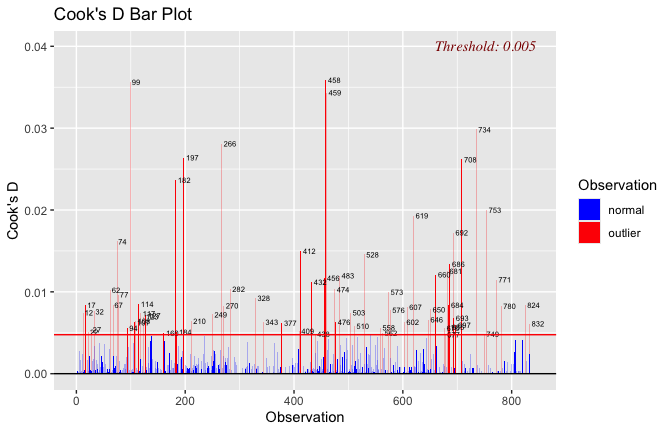
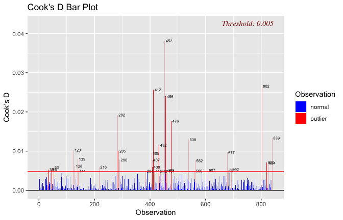
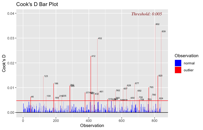
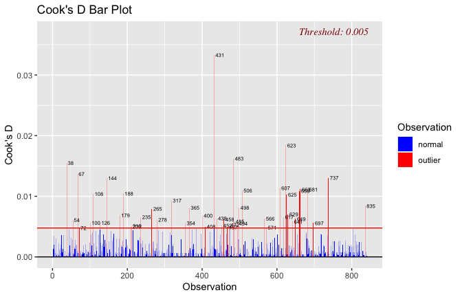
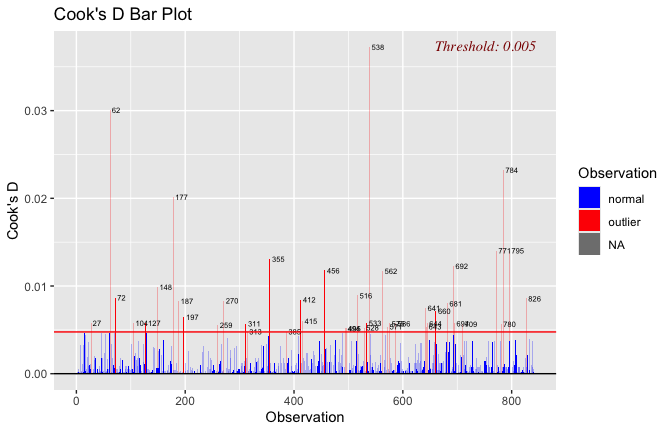
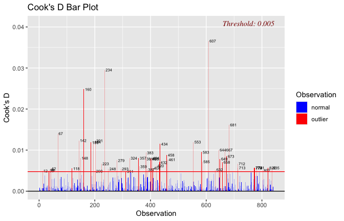
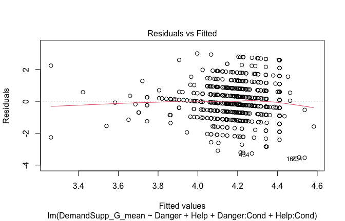
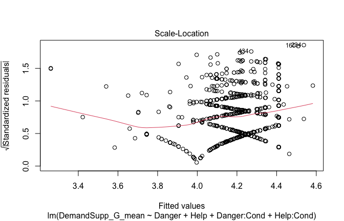
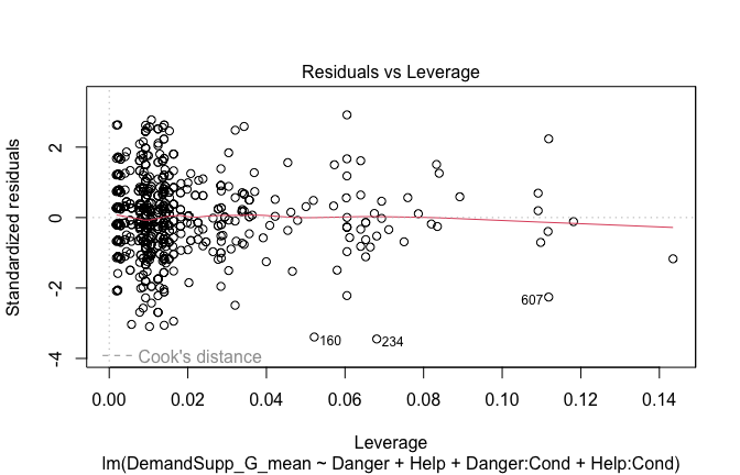
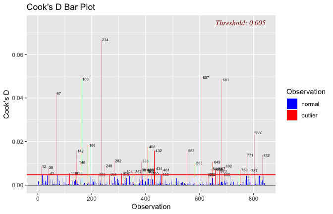
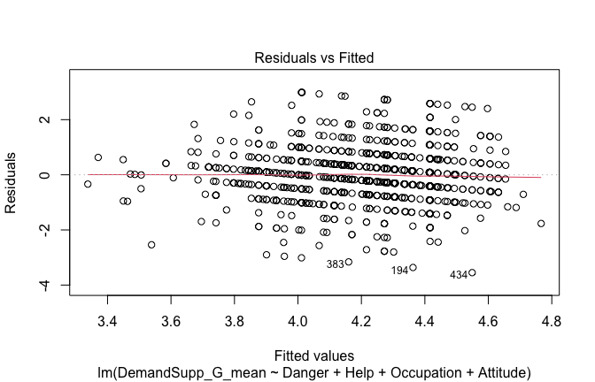
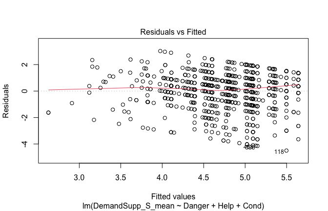
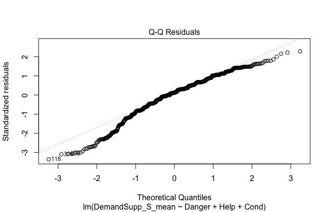
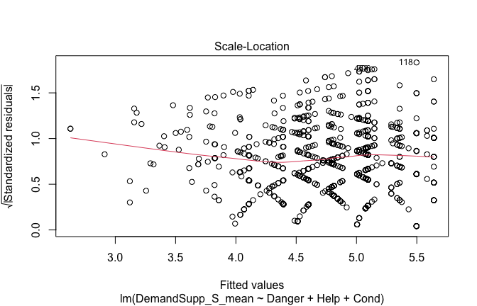
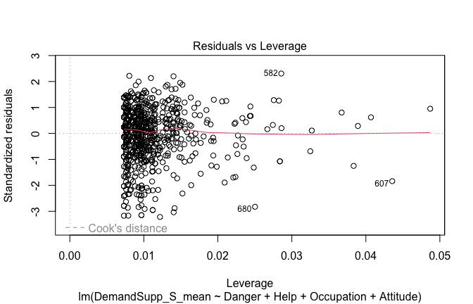
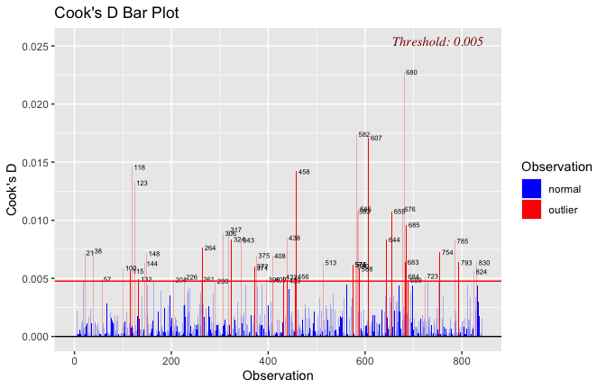
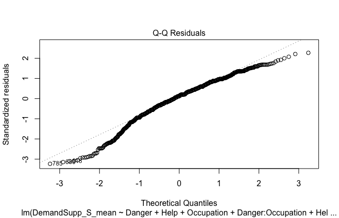
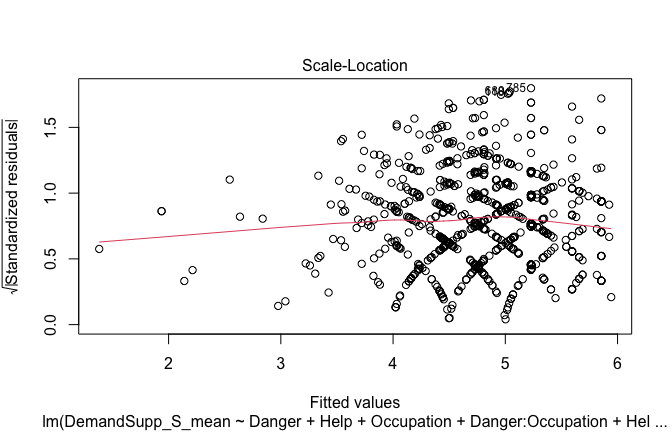
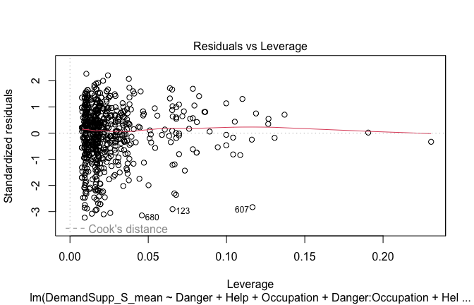
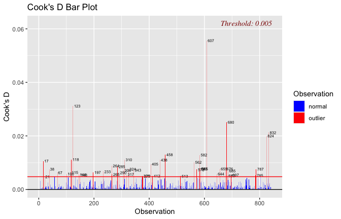
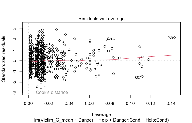
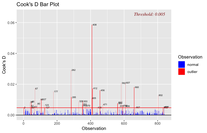
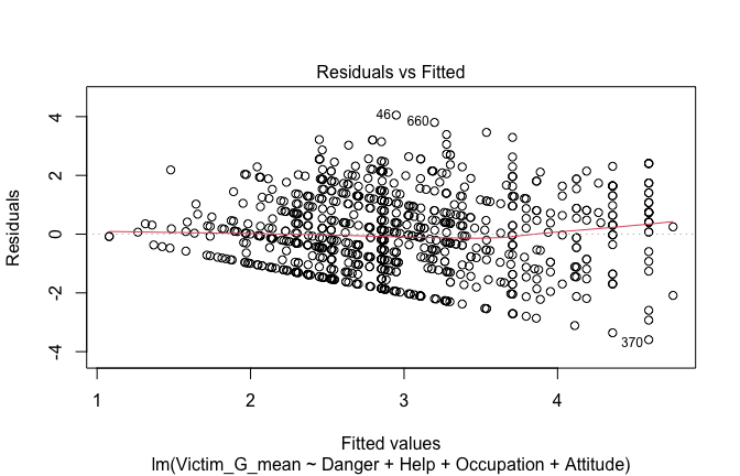
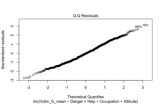
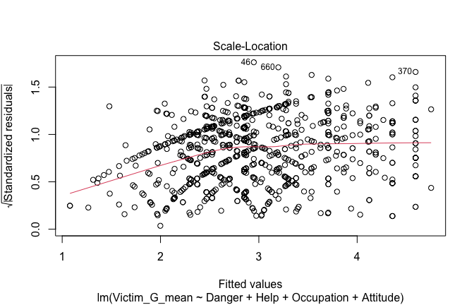
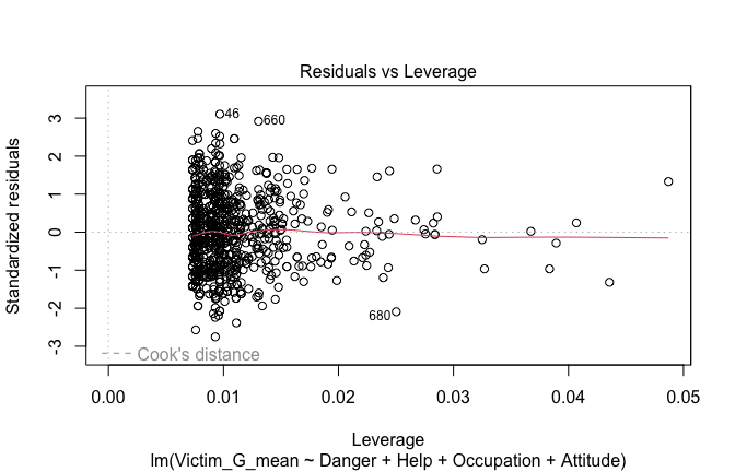
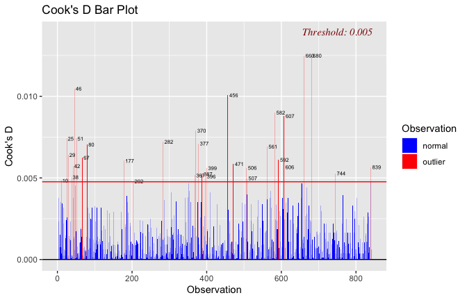
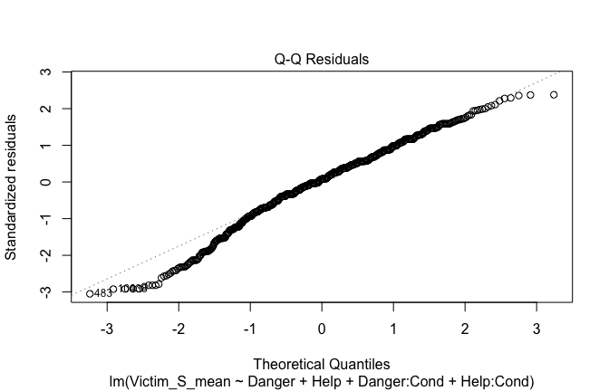
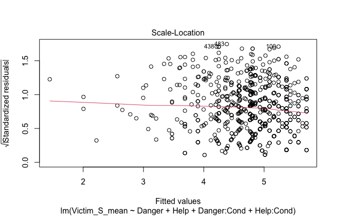
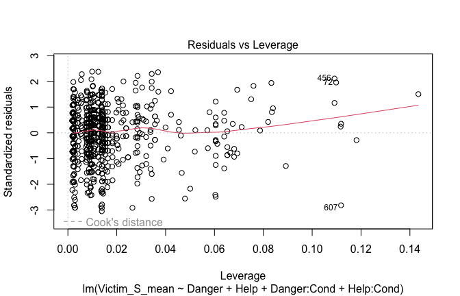
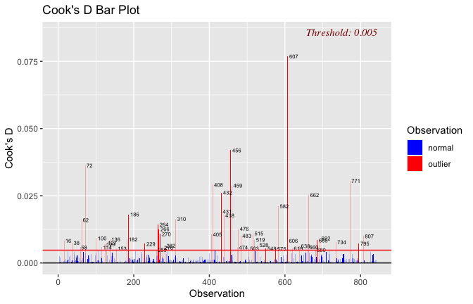
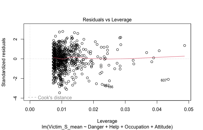
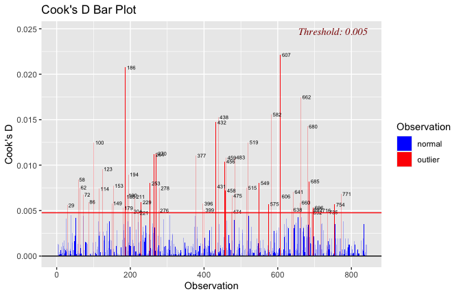
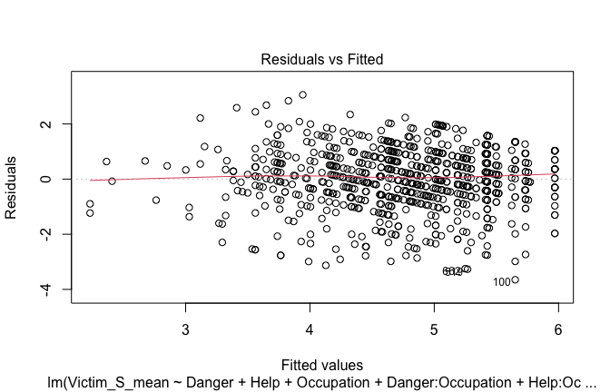
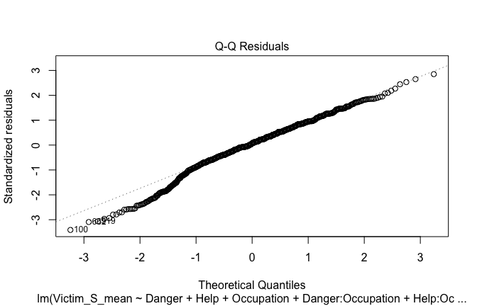
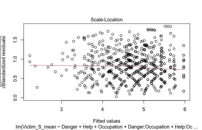
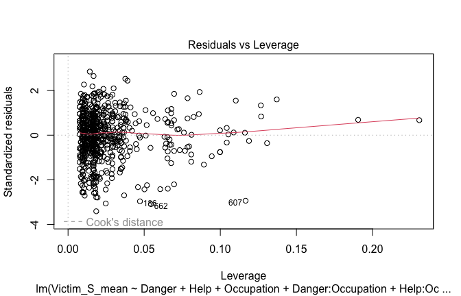
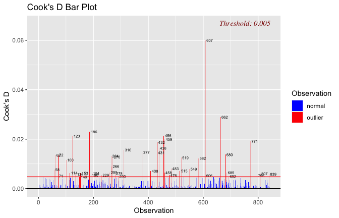
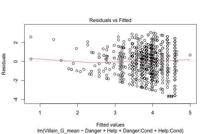
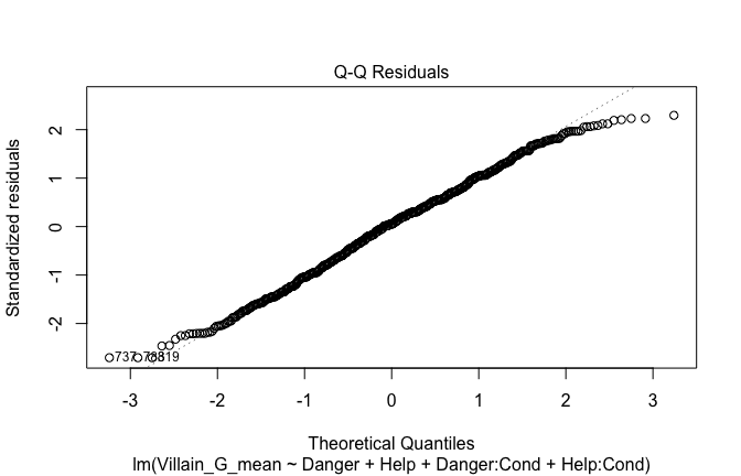
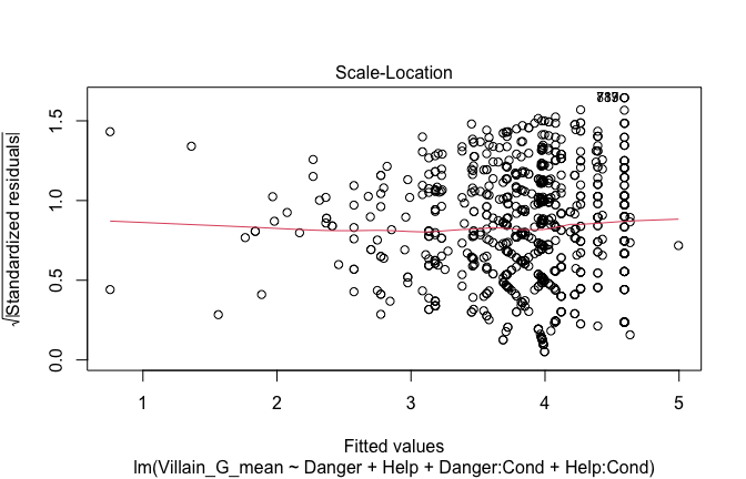
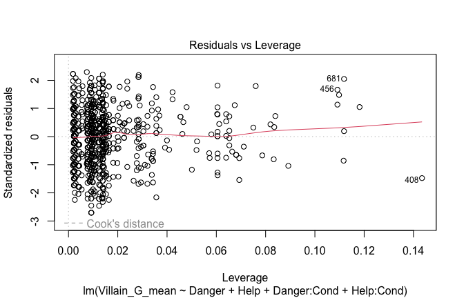
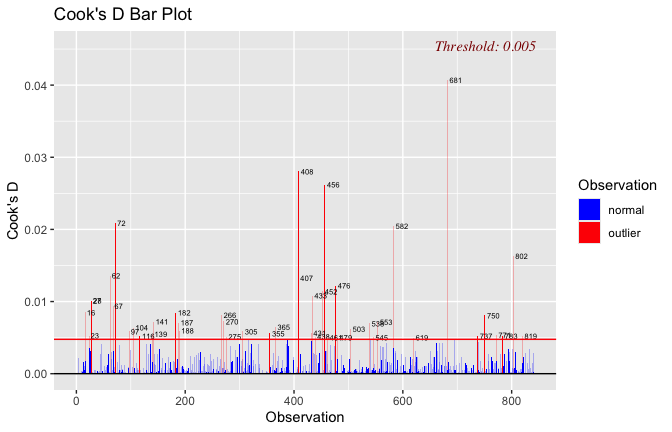
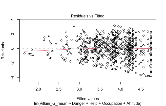
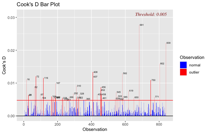
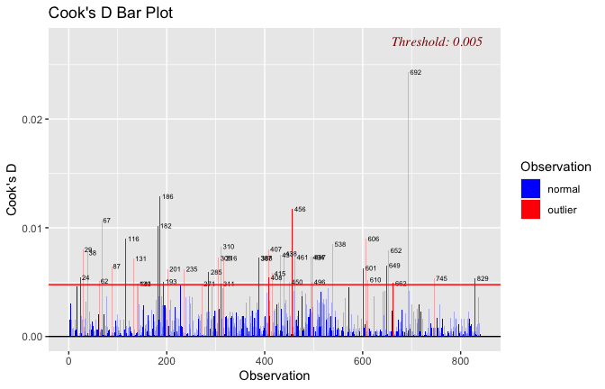
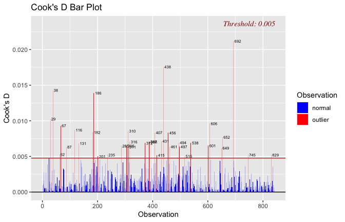
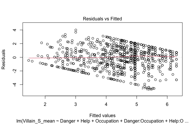
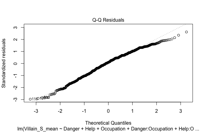
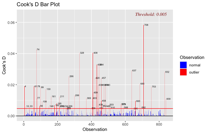
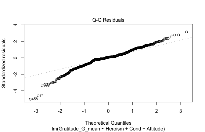
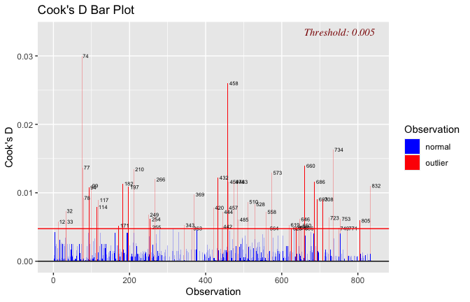
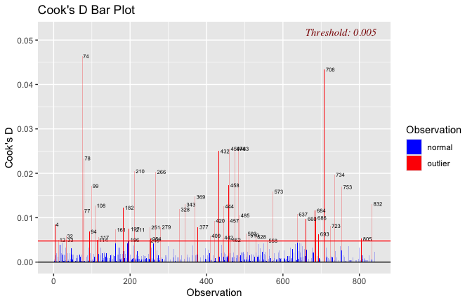
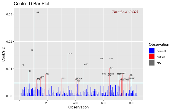
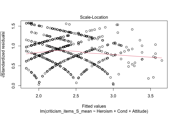
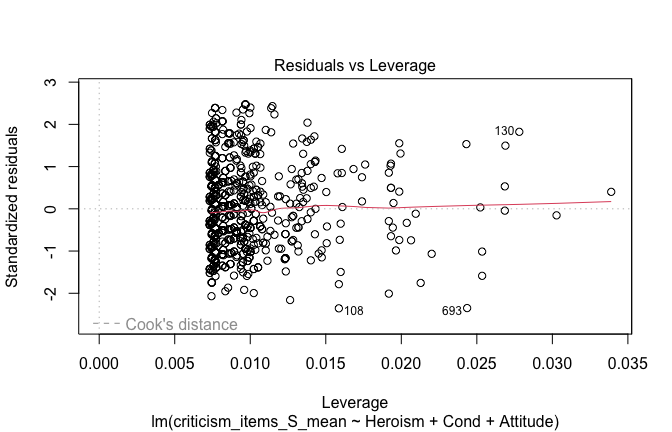
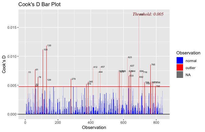
Toggle details of the models diagnostics and outlier analyses

We scale all numeric variables, and we add our sum-to-zero contrast to the occupation level.

scale_scores <- stacked_num[, c(40, 2, 48:57, 36:39, 34, 35)]
scale_scores$Cond <- as.factor(scale_scores$Cond)
contrasts(scale_scores$Cond) <- contr.sum(nlevels(scale_scores$Cond))
contrasts(scale_scores$Cond) # Deviations from registration!! We need to use sum to zero contrasts to make coef interpretable

##             [,1] [,2] [,3] [,4] [,5]
## Firefighter    1    0    0    0    0
## Journalist     0    1    0    0    0
## Nurse          0    0    1    0    0
## Psych          0    0    0    1    0
## Soldier        0    0    0    0    1
## Weld          -1   -1   -1   -1   -1

scale_scores$Heroism <- scale_scores$HW_1
scale_scores$Attitude <- scale(scale_scores$AttW)
scale_scores$Danger <- scale(scale_scores$DangerHelpW_1)
scale_scores$Help <- scale(scale_scores$DangerHelpW_2)

H1: Heroism is positively associated to gratitude

We are grateful for our heroes. As such, at a general level, people might declare openly gratefulness toward workers, and at the specific level, they are likely to display public support for the workers that are heroised. Sharing supportive post online, donating to campaigns, volunteering their time… people want to give back to heroes.

General level

To what extent do you feel grateful for XXXs’ work?

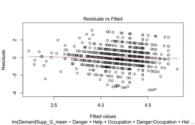
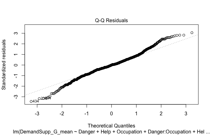
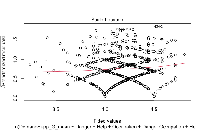
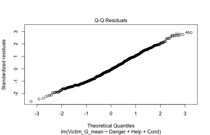
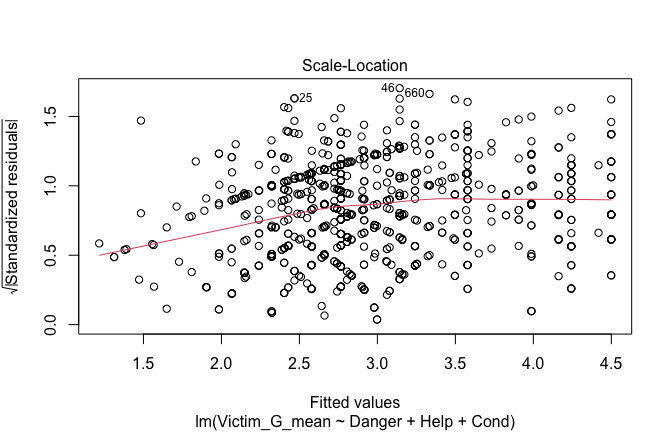
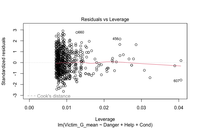
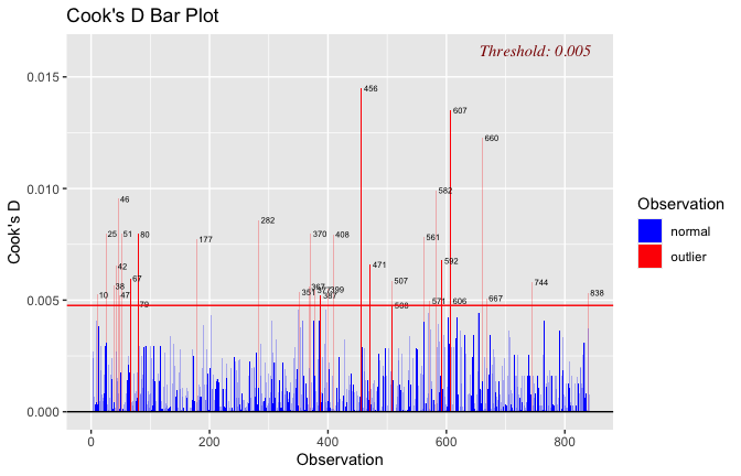
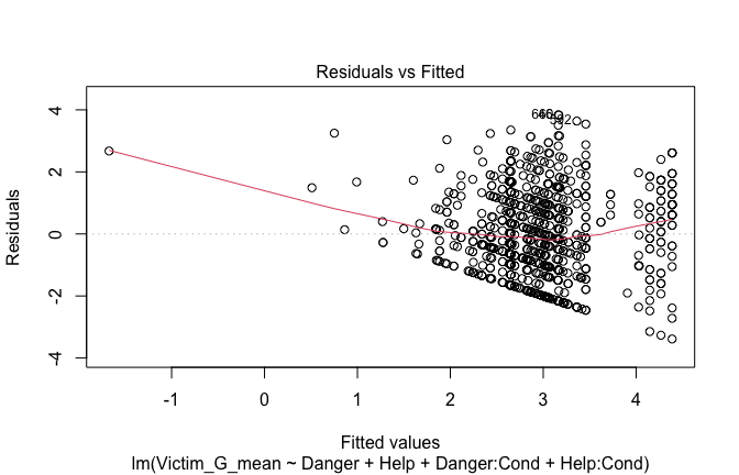
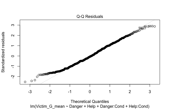
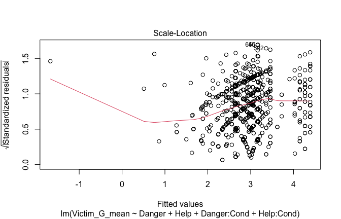
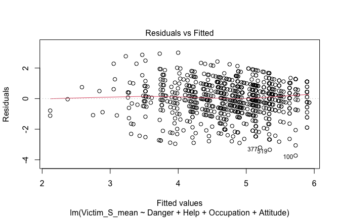
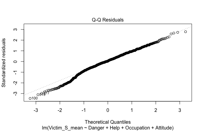
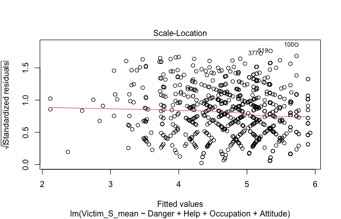
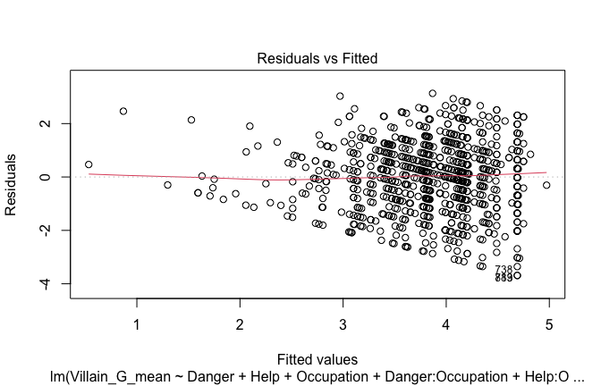
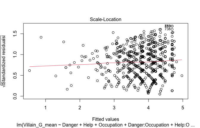
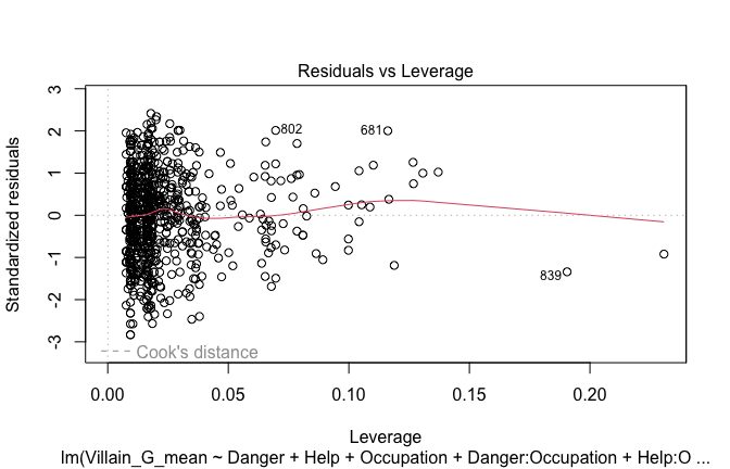
Toggle details of the models diagnostics and outlier analyses

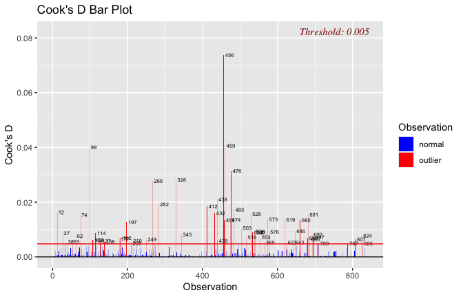
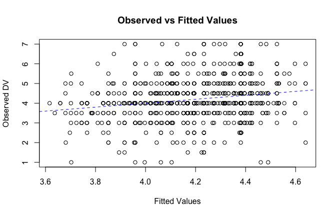
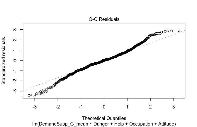
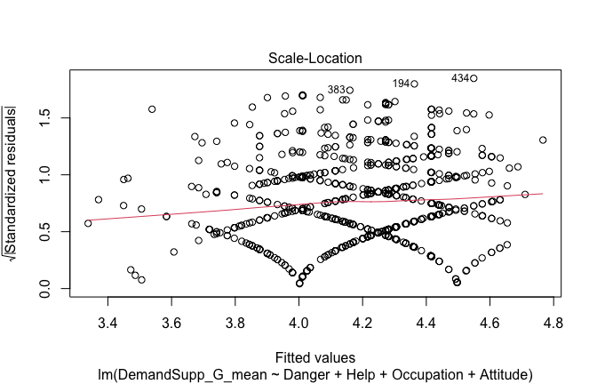
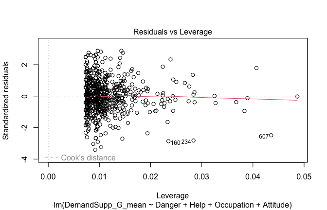
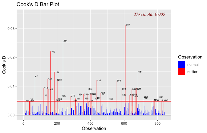
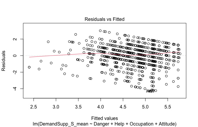
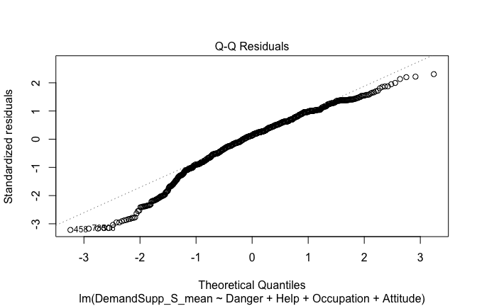
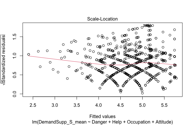
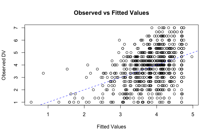
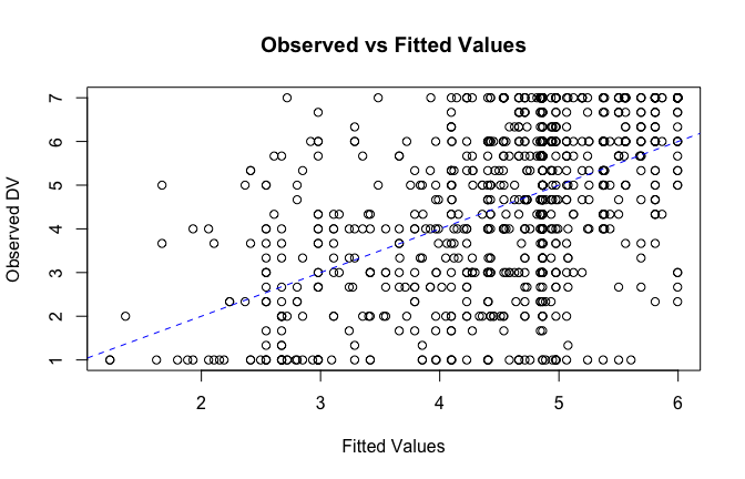
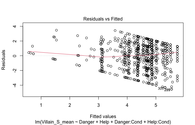
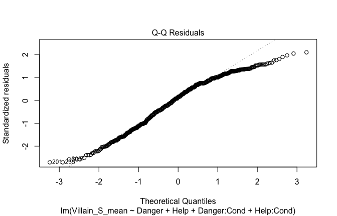
Below, you’ll find model diagnostics (QQ plot, fitted vs residuals, linearity), Outliers analysis, and more details on the output

[NOTE THAT EFFECT SIZES REPORTED IN THE REPORT COMMANDS BELOW SHOULD NOT BE TRUSTED]

paste0("####################################################")

## [1] "####################################################"

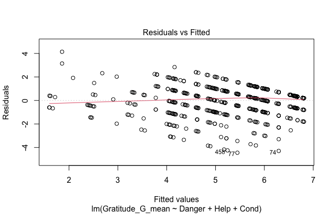
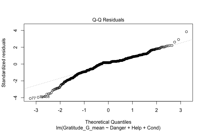
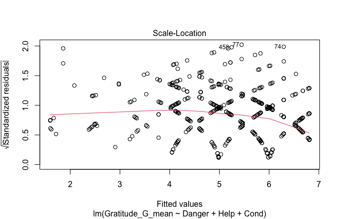
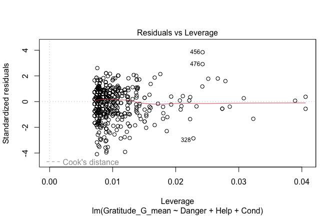
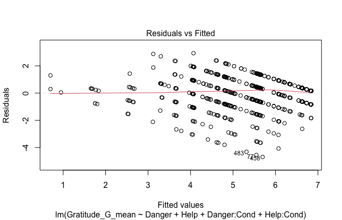
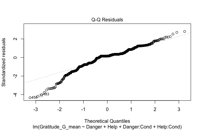
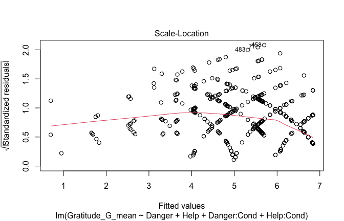
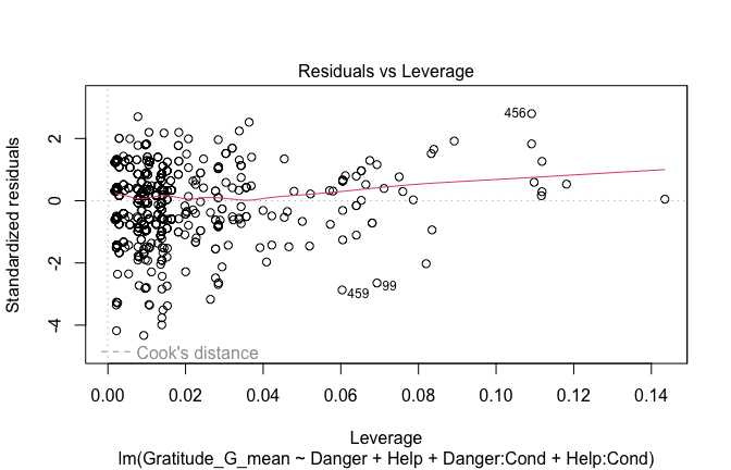
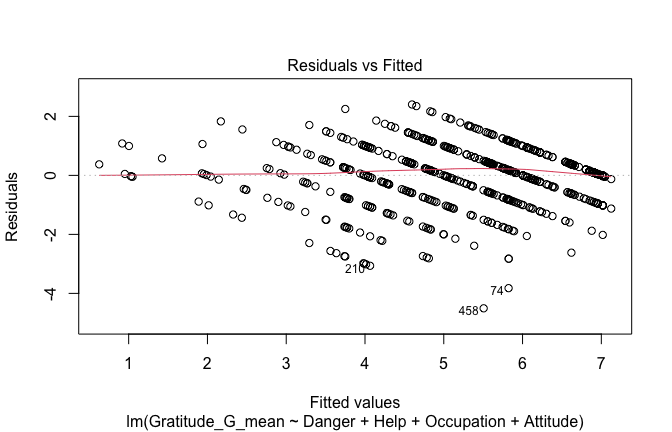
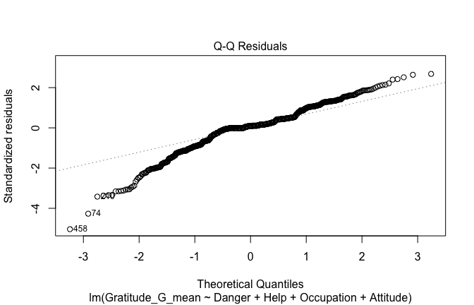
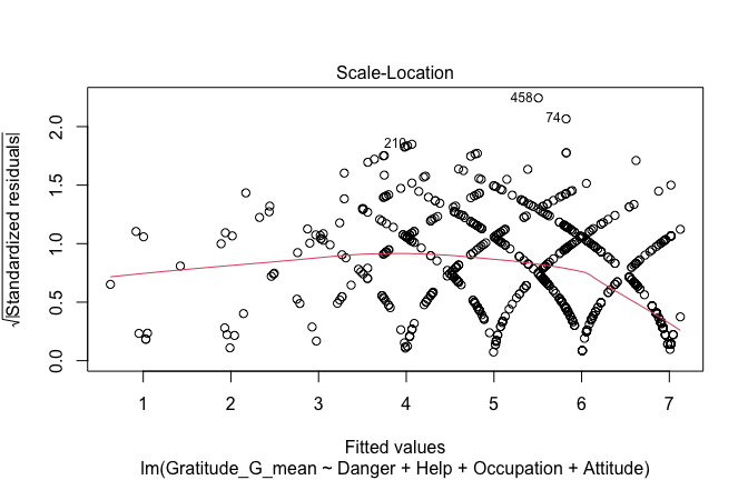
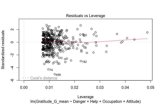
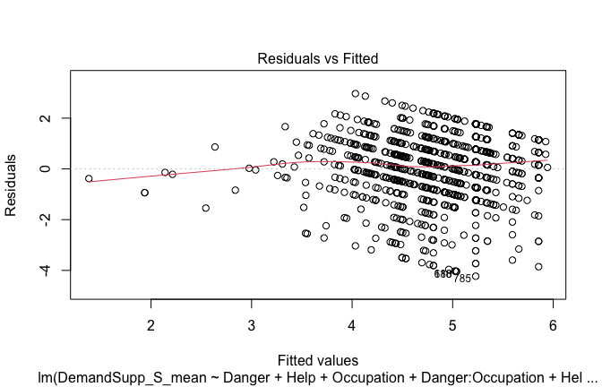
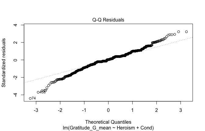
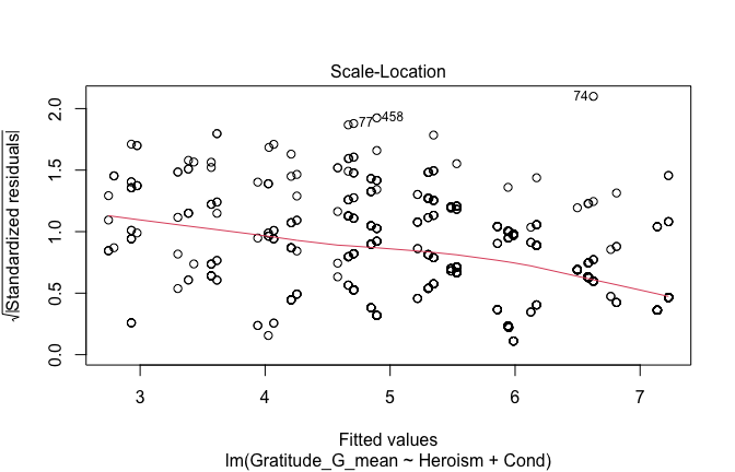
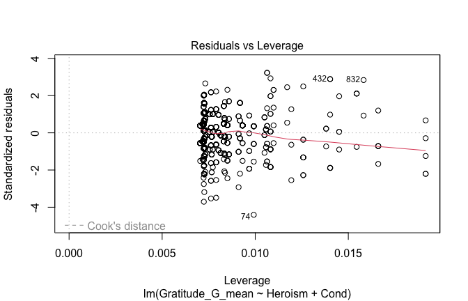
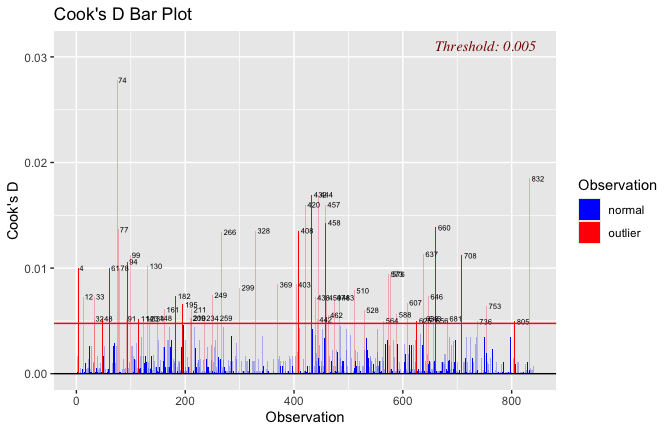
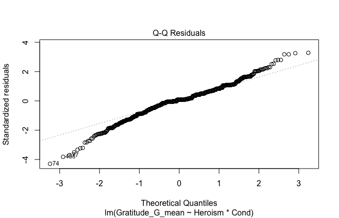
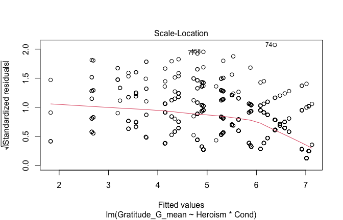
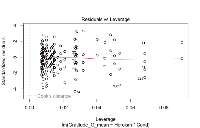
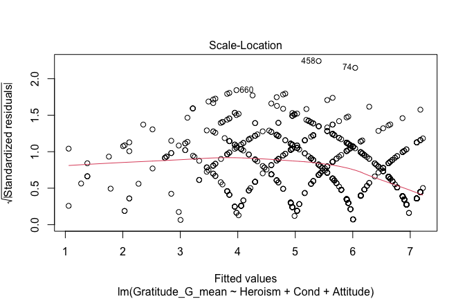
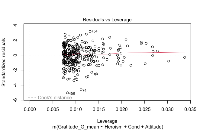
paste0("Diagnostics for Model 1: DV ~ Heroism + Occupation")

## [1] "Diagnostics for Model 1: DV ~ Heroism + Occupation"

paste0("####################################################")

## [1] "####################################################"

mod1 <- lm(Gratitude_G_mean ~ Heroism  + Cond, data = scale_scores)
mod1r <- lmrob(Gratitude_G_mean ~ Heroism  + Cond, data = scale_scores)
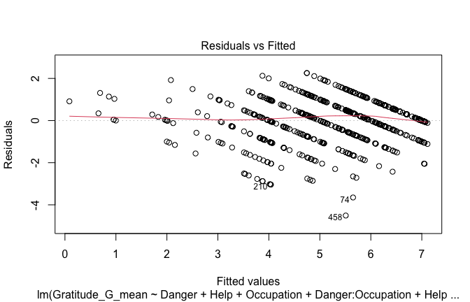
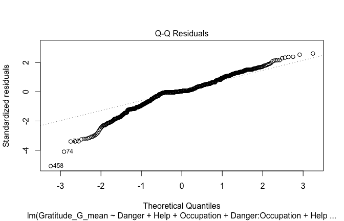
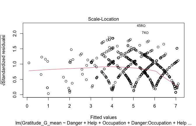
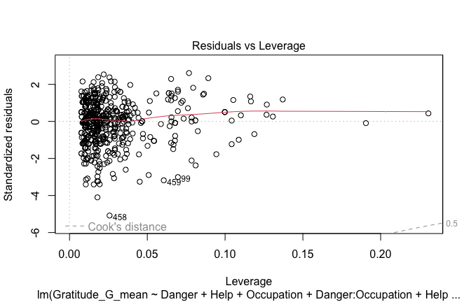
plot(mod1)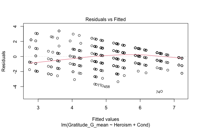

ols_plot_cooksd_bar(mod1, type = 1)

paste0("Comparison with Robust model")

## [1] "Comparison with Robust model"

models <- list("OLS (lm)" = mod1, "Robust (lmrob)" = mod1r)
modelsummary(
  models,
  statistic = c("({std.error})", "{statistic}", "p = {p.value}"),
  gof_omit  = "IC|Log.Lik",   # robust AIC comparability is iffy; omit by default
  output    = "html"
)

	OLS (lm)	Robust (lmrob)
(Intercept)	2.383	2.264
	(0.128)	(0.222)
	18.555	10.211
	p = <0.001	p = <0.001
Heroism	0.639	0.669
	(0.025)	(0.038)
	25.560	17.402
	p = <0.001	p = <0.001
Cond1	0.369	0.305
	(0.085)	(0.067)
	4.345	4.537
	p = <0.001	p = <0.001
Cond2	−0.093	−0.097
	(0.088)	(0.110)
	−1.054	−0.876
	p = 0.292	p = 0.381
Cond3	0.279	0.201
	(0.083)	(0.067)
	3.361	2.989
	p = <0.001	p = 0.003
Cond4	−0.047	−0.073
	(0.082)	(0.090)
	−0.575	−0.807
	p = 0.565	p = 0.420
Cond5	−0.276	−0.198
	(0.082)	(0.088)
	−3.365	−2.253
	p = <0.001	p = 0.025
Num.Obs.	840	840
R2	0.546	0.609
R2 Adj.	0.542	0.606
RMSE	1.05	1.05

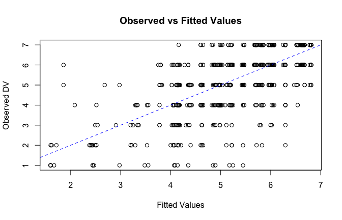
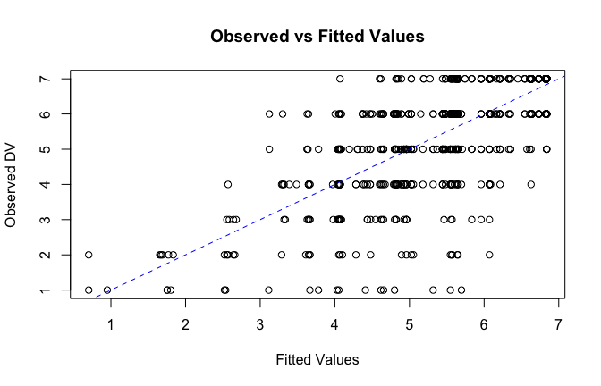
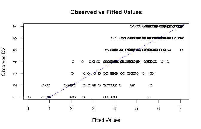
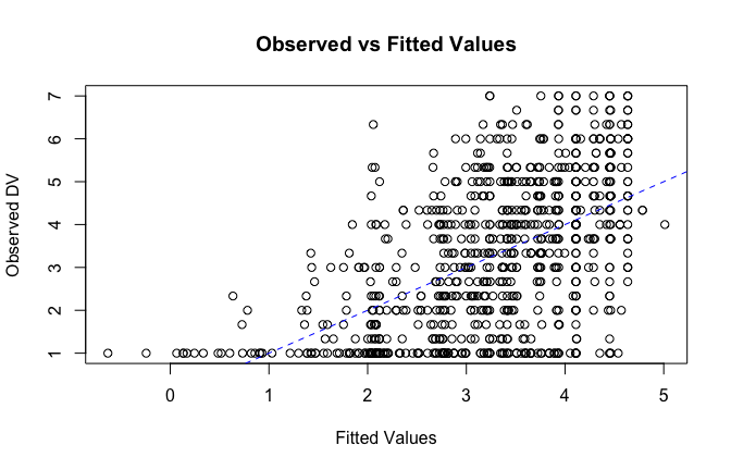
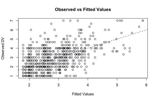
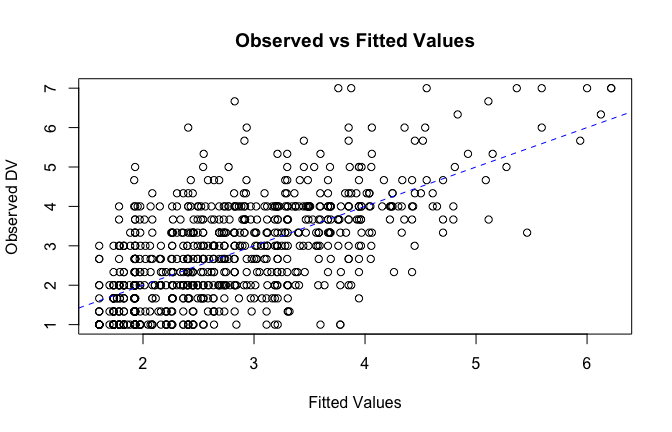
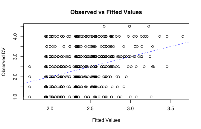
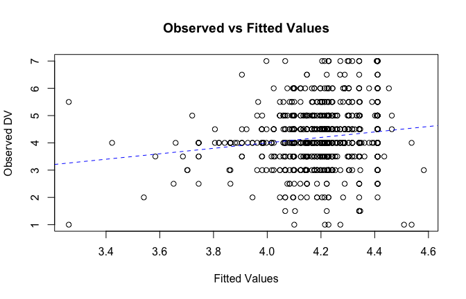
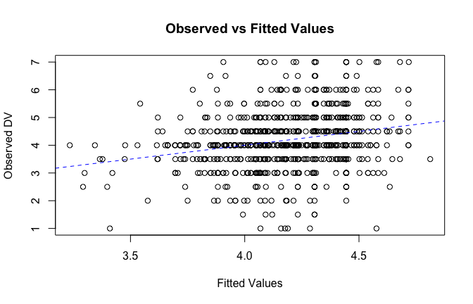
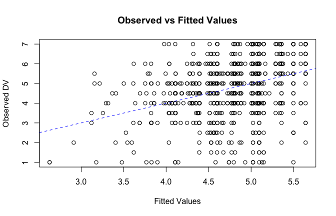
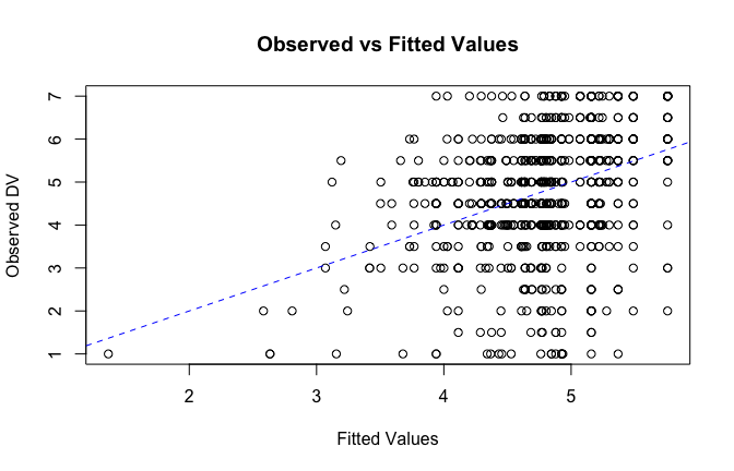
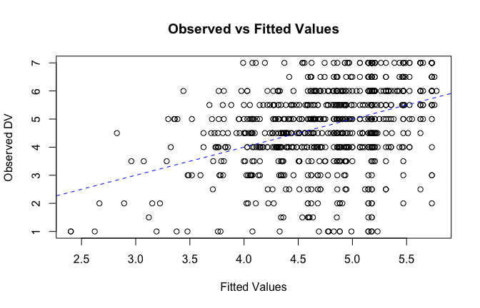
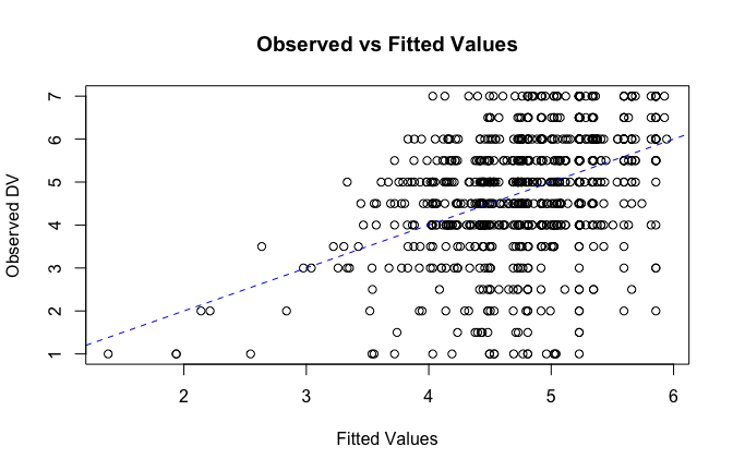
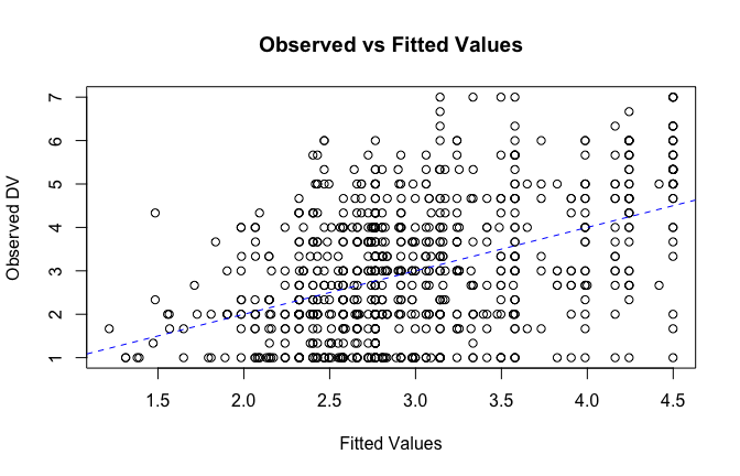
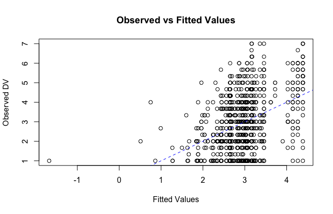
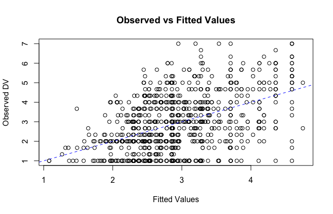
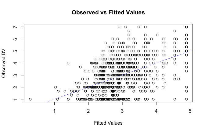
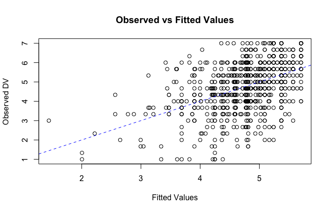
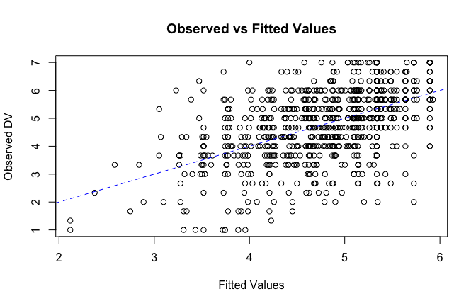
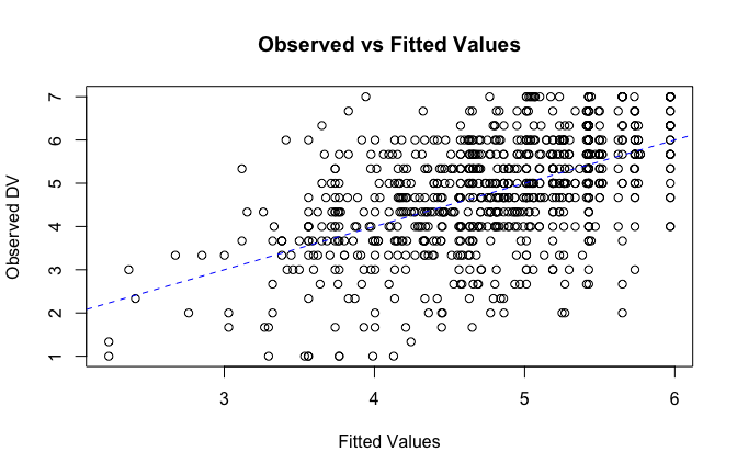
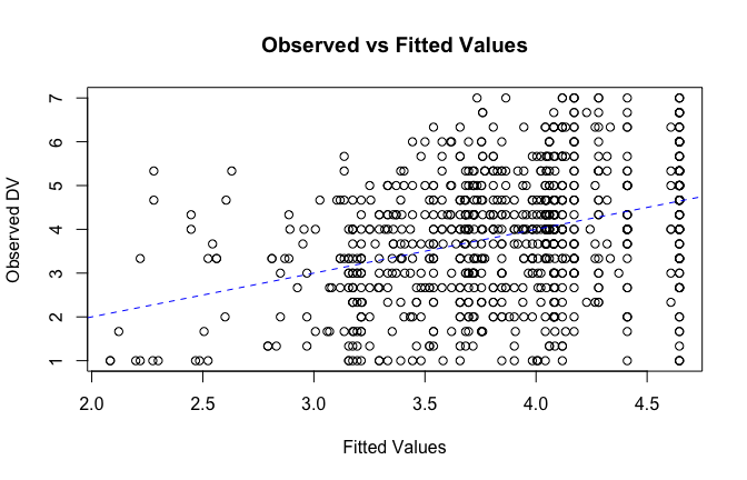
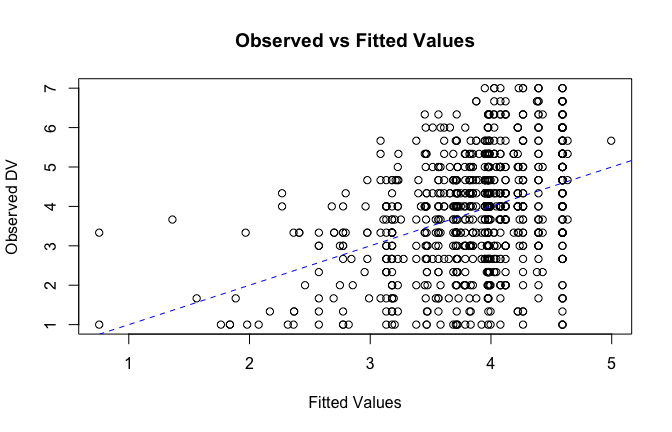
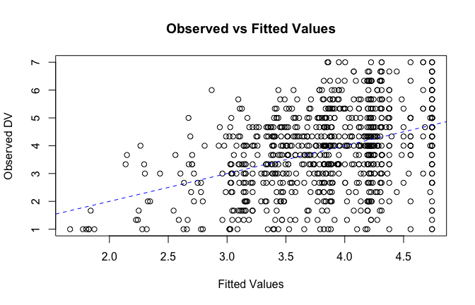
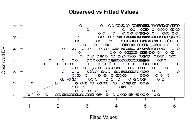
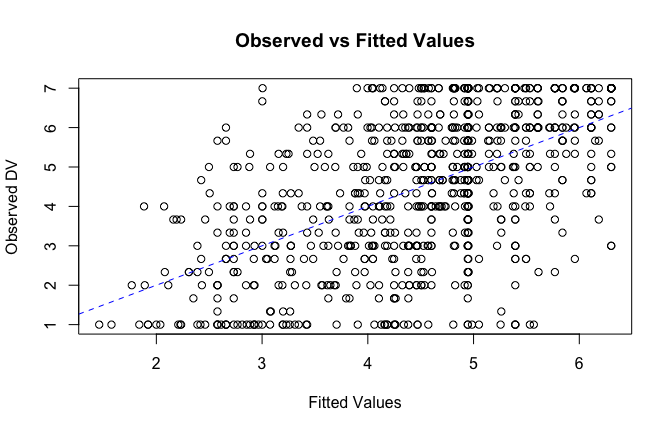
fitted_vals <- fitted(mod1)

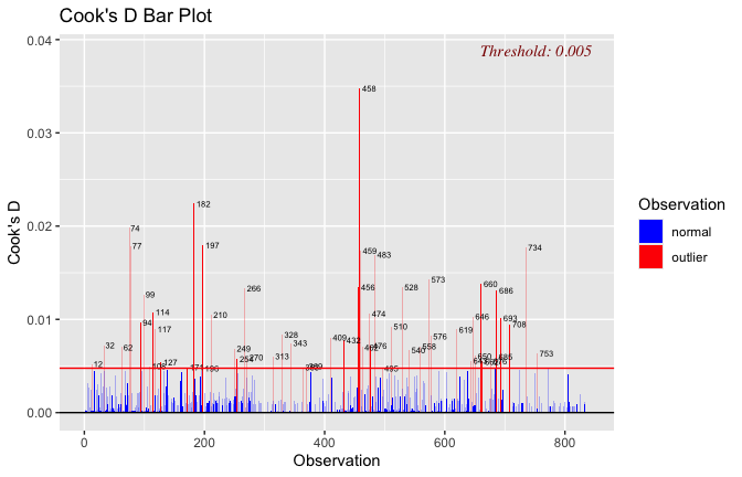
# Plot observed values against fitted values
plot(fitted_vals, scale_scores$Gratitude_G_mean,
     xlab = "Fitted Values",
     ylab = "Observed DV",
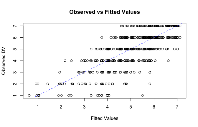
     main = "Observed vs Fitted Values")
abline(0, 1, col = "blue", lty = 2)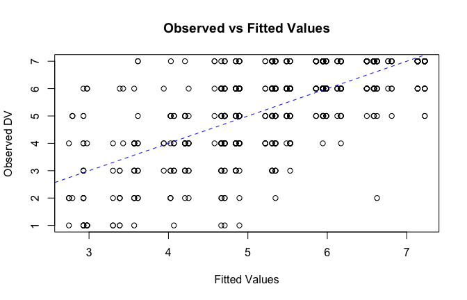

paste0("####################################################")

## [1] "####################################################"

paste0("Diagnostics for Model 2: DV ~ Heroism * Occupation")

## [1] "Diagnostics for Model 2: DV ~ Heroism * Occupation"

paste0("####################################################")

## [1] "####################################################"

mod1 <- lm(Gratitude_G_mean ~ Heroism  * Cond, data = scale_scores)
mod1r <- lmrob(Gratitude_G_mean ~ Heroism  * Cond, data = scale_scores)
plot(mod1)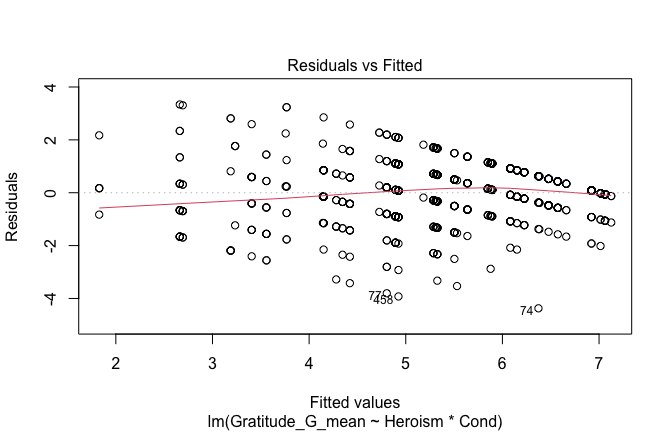

ols_plot_cooksd_bar(mod1, type = 1)

paste0("Comparison with Robust model")

## [1] "Comparison with Robust model"

models <- list("OLS (lm)" = mod1, "Robust (lmrob)" = mod1r)
modelsummary(
  models,
  statistic = c("({std.error})", "{statistic}", "p = {p.value}"),
  gof_omit  = "IC|Log.Lik",   # robust AIC comparability is iffy; omit by default
  output    = "html"
)

	OLS (lm)	Robust (lmrob)
(Intercept)	2.611	2.596
	(0.133)	(0.210)
	19.674	12.379
	p = <0.001	p = <0.001
Heroism	0.607	0.626
	(0.025)	(0.037)
	24.080	17.059
	p = <0.001	p = <0.001
Cond1	1.877	2.536
	(0.397)	(0.440)
	4.731	5.760
	p = <0.001	p = <0.001
Cond2	−0.693	−0.929
	(0.226)	(0.323)
	−3.071	−2.875
	p = 0.002	p = 0.004
Cond3	0.364	0.667
	(0.295)	(0.546)
	1.233	1.222
	p = 0.218	p = 0.222
Cond4	−0.001	−0.592
	(0.266)	(0.605)
	−0.004	−0.978
	p = 0.996	p = 0.328
Cond5	−1.647	−1.794
	(0.265)	(0.344)
	−6.205	−5.220
	p = <0.001	p = <0.001
Heroism × Cond1	−0.259	−0.372
	(0.067)	(0.070)
	−3.891	−5.324
	p = <0.001	p = <0.001
Heroism × Cond2	0.137	0.175
	(0.054)	(0.067)
	2.559	2.596
	p = 0.011	p = 0.010
Heroism × Cond3	−0.023	−0.089
	(0.052)	(0.086)
	−0.448	−1.035
	p = 0.654	p = 0.301
Heroism × Cond4	−0.028	0.082
	(0.055)	(0.114)
	−0.515	0.717
	p = 0.607	p = 0.473
Heroism × Cond5	0.258	0.273
	(0.050)	(0.055)
	5.168	4.941
	p = <0.001	p = <0.001
Num.Obs.	840	840
R2	0.567	0.660
R2 Adj.	0.562	0.655
RMSE	1.02	1.03

fitted_vals <- fitted(mod1)

# Plot observed values against fitted values
plot(fitted_vals, scale_scores$Gratitude_G_mean,
     xlab = "Fitted Values",
     ylab = "Observed DV",
     main = "Observed vs Fitted Values")
abline(0, 1, col = "blue", lty = 2)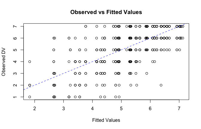

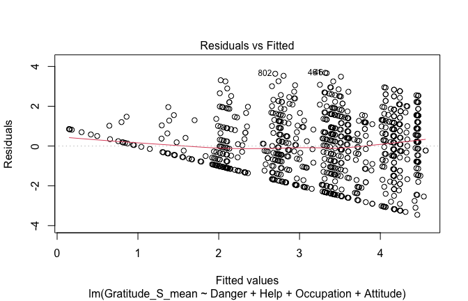
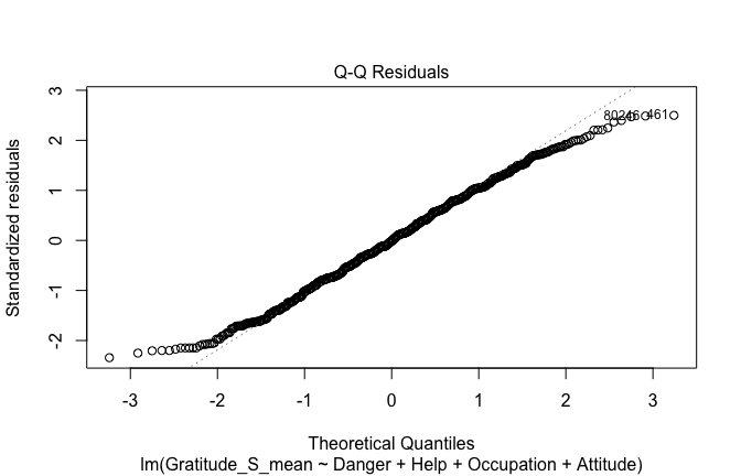
paste0("####################################################")

## [1] "####################################################"

paste0("Diagnostics for Model 3: DV ~ Heroism + Occupation + Attitude")

## [1] "Diagnostics for Model 3: DV ~ Heroism + Occupation + Attitude"

paste0("####################################################")

## [1] "####################################################"

mod1 <- lm(Gratitude_G_mean ~ Heroism  + Cond + Attitude, data = scale_scores)
mod1r <- lmrob(Gratitude_G_mean ~ Heroism  + Cond + Attitude, data = scale_scores)

## Warning in lmrob.S(x, y, control = control): S-estimated scale == 0: Probably
## exact fit; check your data

## Warning in lmrob.fit(x, y, control, init = init): initial estim. 'init' not
## converged -- will be return()ed basically unchanged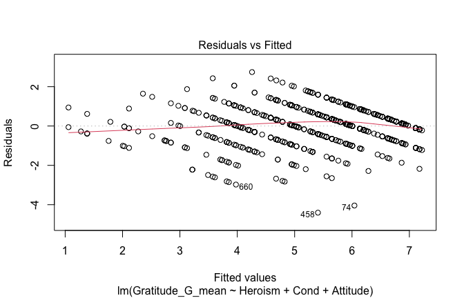

plot(mod1)

ols_plot_cooksd_bar(mod1, type = 1)

paste0("Comparison with Robust model")

## [1] "Comparison with Robust model"

models <- list("OLS (lm)" = mod1, "Robust (lmrob)" = mod1r)
modelsummary(
  models,
  statistic = c("({std.error})", "{statistic}", "p = {p.value}"),
  gof_omit  = "IC|Log.Lik",   # robust AIC comparability is iffy; omit by default
  output    = "html"
)

	OLS (lm)	Robust (lmrob)
(Intercept)	4.337	5.839
	(0.148)	(0.000)
	29.250
	p = <0.001
Heroism	0.243	−0.000
	(0.029)	(0.000)
	8.249
	p = <0.001
Cond1	0.169	−0.167
	(0.072)	(0.000)
	2.363
	p = 0.018
Cond2	0.213	0.833
	(0.075)	(0.000)
	2.831
	p = 0.005
Cond3	0.106	−0.167
	(0.070)	(0.000)
	1.511
	p = 0.131
Cond4	−0.142	−0.167
	(0.068)	(0.000)
	−2.071
	p = 0.039
Cond5	−0.112	−0.167
	(0.069)	(0.000)
	−1.620
	p = 0.106
Attitude	0.943	1.291
	(0.049)	(0.000)
	19.073
	p = <0.001
Num.Obs.	840	840
R2	0.684	1.000
R2 Adj.	0.681	1.000
RMSE	0.88	1.02

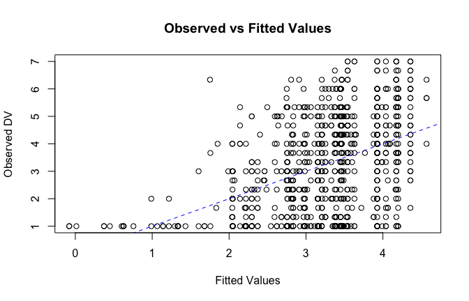
fitted_vals <- fitted(mod1)

# Plot observed values against fitted values
plot(fitted_vals, scale_scores$Gratitude_G_mean,
     xlab = "Fitted Values",
     ylab = "Observed DV",
     main = "Observed vs Fitted Values")
abline(0, 1, col = "blue", lty = 2)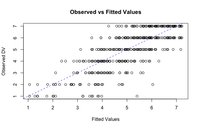

paste0("####################################################")

## [1] "####################################################"

paste0("Diagnostics for Model 4: DV ~ Heroism * Occupation + Attitude")

## [1] "Diagnostics for Model 4: DV ~ Heroism * Occupation + Attitude"

paste0("####################################################")

## [1] "####################################################"

mod1 <- lm(Gratitude_G_mean ~ Heroism*Cond + Attitude, data = scale_scores)
mod1r <- lmrob(Gratitude_G_mean ~ Heroism*Cond + Attitude, data = scale_scores)

## Warning in lmrob.S(x, y, control = control): find_scale() did not converge in
## 'maxit.scale' (= 200) iterations with tol=1e-10, last rel.diff=0

## Warning in lmrob.S(x, y, control = control): find_scale() did not converge in
## 'maxit.scale' (= 200) iterations with tol=1e-10, last rel.diff=0

## Warning in lmrob.fit(x, y, control, init = init): M-step did NOT converge.
## Returning unconverged SM-estimate

plot(mod1)

ols_plot_cooksd_bar(mod1, type = 1)

paste0("Comparison with Robust model")

## [1] "Comparison with Robust model"

models <- list("OLS (lm)" = mod1, "Robust (lmrob)" = mod1r)
modelsummary(
  models,
  statistic = c("({std.error})", "{statistic}", "p = {p.value}"),
  gof_omit  = "IC|Log.Lik",   # robust AIC comparability is iffy; omit by default
  output    = "html"
)

	OLS (lm)	Robust (lmrob)
(Intercept)	4.391	4.892
	(0.150)
	29.367
	p = <0.001
Heroism	0.239	0.165
	(0.030)
	8.105
	p = <0.001
Cond1	1.163	0.786
	(0.338)
	3.435
	p = <0.001
Cond2	0.015	−0.470
	(0.195)
	0.079
	p = 0.937
Cond3	0.104	0.142
	(0.251)
	0.413
	p = 0.680
Cond4	−0.295	0.360
	(0.226)
	−1.306
	p = 0.192
Cond5	−0.832	−0.680
	(0.229)
	−3.626
	p = <0.001
Attitude	0.908	0.963
	(0.050)
	18.063
	p = <0.001
Heroism × Cond1	−0.168	−0.116
	(0.057)
	−2.972
	p = 0.003
Heroism × Cond2	0.036	0.111
	(0.046)
	0.780
	p = 0.435
Heroism × Cond3	−0.002	−0.022
	(0.044)
	−0.056
	p = 0.955
Heroism × Cond4	0.025	−0.083
	(0.047)
	0.545
	p = 0.586
Heroism × Cond5	0.134	0.113
	(0.043)
	3.138
	p = 0.002
Num.Obs.	840	840
R2	0.690	0.849
R2 Adj.	0.685	0.846
RMSE	0.87	0.90

fitted_vals <- fitted(mod1)

# Plot observed values against fitted values
plot(fitted_vals, scale_scores$Gratitude_G_mean,
     xlab = "Fitted Values",
     ylab = "Observed DV",
     main = "Observed vs Fitted Values")
abline(0, 1, col = "blue", lty = 2)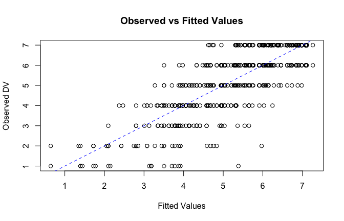

paste0("####################################################")

## [1] "####################################################"

paste0("REPORTS for each model (please ignore the eta squares, they are way off")

## [1] "REPORTS for each model (please ignore the eta squares, they are way off"

paste0("####################################################")

## [1] "####################################################"

paste0("MODEL 1: Gratitude_G_mean ~ Heroism")

## [1] "MODEL 1: Gratitude_G_mean ~ Heroism"

report(Anova(mod1 <- lm(Gratitude_G_mean ~ Heroism  + Cond, data = scale_scores), type = "III"))

## The ANOVA suggests that:
## 
##   - The main effect of Heroism is statistically significant and large (F(1, 833)
## = 653.30, p < .001; Eta2 (partial) = 0.44, 95% CI [0.40, 1.00])
##   - The main effect of Cond is statistically significant and small (F(5, 833) =
## 8.16, p < .001; Eta2 (partial) = 0.05, 95% CI [0.02, 1.00])
## 
## Effect sizes were labelled following Field's (2013) recommendations.

paste0("MODEL 2: Gratitude_G_mean ~ Heroism * Cond")

## [1] "MODEL 2: Gratitude_G_mean ~ Heroism * Cond"

report(Anova(mod2 <- lm(Gratitude_G_mean ~ Heroism * Cond, data = scale_scores), type = "III"))

## Type 3 ANOVAs only give sensible and informative results when covariates
##   are mean-centered and factors are coded with orthogonal contrasts (such
##   as those produced by `contr.sum`, `contr.poly`, or `contr.helmert`, but
##   *not* by the default `contr.treatment`).

## The ANOVA suggests that:
## 
##   - The main effect of Heroism is statistically significant and large (F(1, 828)
## = 579.85, p < .001; Eta2 (partial) = 0.41, 95% CI [0.37, 1.00])
##   - The main effect of Cond is statistically significant and medium (F(5, 828) =
## 11.07, p < .001; Eta2 (partial) = 0.06, 95% CI [0.03, 1.00])
##   - The interaction between Heroism and Cond is statistically significant and
## small (F(5, 828) = 8.31, p < .001; Eta2 (partial) = 0.05, 95% CI [0.02, 1.00])
## 
## Effect sizes were labelled following Field's (2013) recommendations.

paste0("MODEL 3: Gratitude_G_mean ~ Heroism +scale(Attitude)")

## [1] "MODEL 3: Gratitude_G_mean ~ Heroism +scale(Attitude)"

report(Anova(mod3 <- lm(Gratitude_G_mean ~ Heroism   + Cond +scale(Attitude) , data = scale_scores), type = "III"))

## The ANOVA suggests that:
## 
##   - The main effect of Heroism is statistically significant and medium (F(1, 832)
## = 68.04, p < .001; Eta2 (partial) = 0.08, 95% CI [0.05, 1.00])
##   - The main effect of Cond is statistically significant and small (F(5, 832) =
## 6.24, p < .001; Eta2 (partial) = 0.04, 95% CI [0.01, 1.00])
##   - The main effect of scale(Attitude) is statistically significant and large
## (F(1, 832) = 363.78, p < .001; Eta2 (partial) = 0.30, 95% CI [0.26, 1.00])
## 
## Effect sizes were labelled following Field's (2013) recommendations.

paste0("MODEL 4: Gratitude_G_mean ~ Heroism * Cond + scale(Attitude)")

## [1] "MODEL 4: Gratitude_G_mean ~ Heroism * Cond + scale(Attitude)"

report(Anova(mod4 <-lm(Gratitude_G_mean ~ Heroism * Cond + scale(Attitude), data = scale_scores), type = "III"))

## Type 3 ANOVAs only give sensible and informative results when covariates
##   are mean-centered and factors are coded with orthogonal contrasts (such
##   as those produced by `contr.sum`, `contr.poly`, or `contr.helmert`, but
##   *not* by the default `contr.treatment`).

## The ANOVA suggests that:
## 
##   - The main effect of Heroism is statistically significant and medium (F(1, 827)
## = 65.69, p < .001; Eta2 (partial) = 0.07, 95% CI [0.05, 1.00])
##   - The main effect of Cond is statistically significant and small (F(5, 827) =
## 4.21, p < .001; Eta2 (partial) = 0.02, 95% CI [6.49e-03, 1.00])
##   - The main effect of scale(Attitude) is statistically significant and large
## (F(1, 827) = 326.28, p < .001; Eta2 (partial) = 0.28, 95% CI [0.24, 1.00])
##   - The interaction between Heroism and Cond is statistically significant and
## small (F(5, 827) = 3.14, p = 0.008; Eta2 (partial) = 0.02, 95% CI [2.75e-03,
## 1.00])
## 
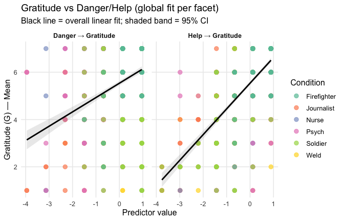
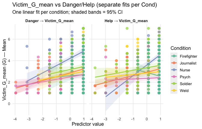
## Effect sizes were labelled following Field's (2013) recommendations.

paste0("Model Comparison: assessing the importance of attitude - not accounting for occupations")

## [1] "Model Comparison: assessing the importance of attitude - not accounting for occupations"

anova(mod1, mod3)

paste0("Model Comparison: assessing the importance of attitude - accounting for occupations")

## [1] "Model Comparison: assessing the importance of attitude - accounting for occupations"

anova(mod2, mod4)

ggplot(scale_scores, aes(y = Gratitude_G_mean, x = Heroism)) +
  # 1) points colored by Cond
  geom_point(aes(color = Cond),
             size = 2.7, alpha = 0.7) +
  
  # 2) ONE global lm line (group = 1 prevents one line per Cond)
  stat_smooth(method = "lm", se = TRUE,
              aes(group = 1),
              color = "black", linewidth = 1) +
  
  # Nice, accessible palette (works well with >3 groups)
  scale_color_brewer(palette = "Set2") +
  
  labs(
    y = "Gratitude (G)",
    x = "Heroism",
    color = "Occupation",
    title = "Heroism vs. Gratitude (G), colored by Occupation",
    subtitle = "Points are participants; black line is overall linear fit with 95% CI"
  ) +
  theme_minimal(base_size = 12) +
  theme(
    legend.position = "right",
    panel.grid.minor = element_blank()
  )

## `geom_smooth()` using formula = 'y ~ x'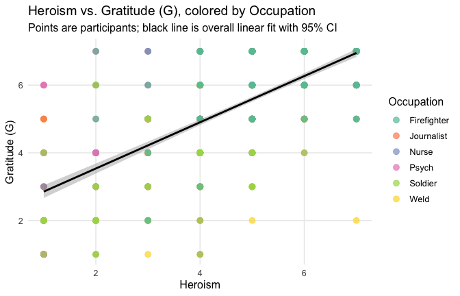

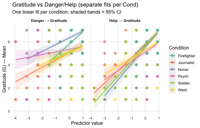
ggplot(scale_scores, aes(y = Gratitude_G_mean, x = Heroism, color = Cond)) +
  # points colored by condition
  geom_point(size = 2.7, alpha = 0.7) +
  # ONE lm line PER condition (because color is mapped here)
  stat_smooth(method = "lm", se = FALSE, linewidth = 1, fullrange = TRUE) +
  scale_color_brewer(palette = "Set2") +
  labs(
    y = "Gratitude (G)",
    x = "Heroism",
    color = "Occupation",
    title = "Heroism vs. Gratitude (G) with per-occupation linear fits"
  ) +
  theme_minimal(base_size = 12) +
  theme(legend.position = "right", panel.grid.minor = element_blank())

## `geom_smooth()` using formula = 'y ~ x'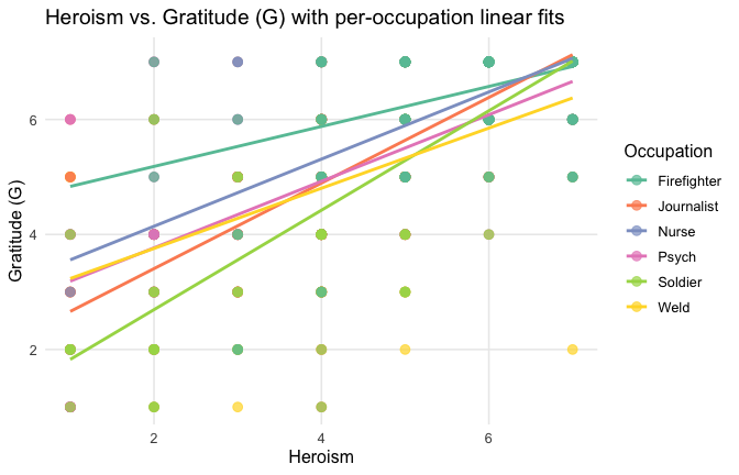

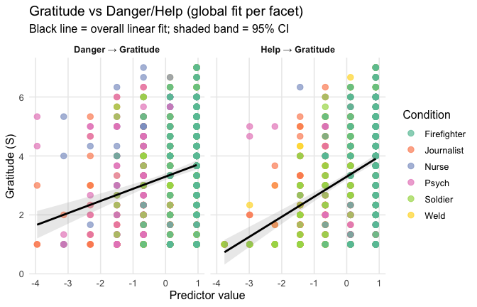
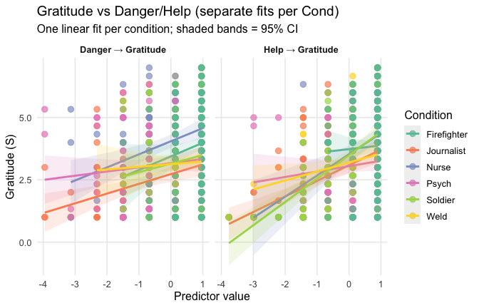
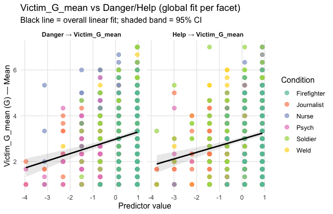
Overall: Heroism predict general gratitude. This is true above and beyond attitude (see Model 3). It is true when controlling for normative effects of occupations (Model 2), and when controlling for both occupations and attitude (Model 4). See Summary tables:

Model 1: “~Heroism + Occupation”

# Make sure Cond is a factor
scale_scores <- scale_scores %>% mutate(Cond = as.factor(Cond))
scale_scores$Occupation <- scale_scores$Cond
scale_scores$Occupation <- as.factor(scale_scores$Occupation)
contrasts(scale_scores$Occupation) <- contr.sum(nlevels(scale_scores$Occupation))


# Partial eta^2 from F and dfs (works for any df1)
eta_p2_fromF <- function(Fval, df1, df2) (Fval * df1) / (Fval * df1 + df2)

tidy_type3 <- function(mod, caption) {
  a <- car::Anova(mod, type = "III")
  tab <- as.data.frame(a)
  tab$Term <- rownames(tab)
  names(tab) <- sub(" ", "_", names(tab))  # "Sum Sq" -> "Sum_Sq", etc.

  resid_df2 <- tab$Df[tab$Term == "Residuals"]

  out <- tab %>%
    dplyr::filter(!(Term %in% c("(Intercept)","Residuals"))) %>%
    dplyr::transmute(
      Term,
      df1   = Df,
      df2   = resid_df2,
      F     = round(F_value, 2),
      p     = ifelse(`Pr(>F)` < .001, "< .001", sprintf("= %.3f", `Pr(>F)`)),
      eta2p = round((F_value * Df) / (F_value * Df + resid_df2), 3)
    )

  kbl <- knitr::kable(out, format = "html", align = "lrrrcr", caption = caption)

  # If kableExtra is installed, add a vertical separator + padding between p and eta2p
  if ("column_spec" %in% getNamespaceExports("kableExtra")) {
    kbl <- kbl %>%
      kableExtra::kable_styling(full_width = FALSE, bootstrap_options = c("striped","hover")) %>%
      # p is column 5 → add a right border and a bit of right padding
      kableExtra::column_spec(5, border_right = "1px solid #ddd",
                                 extra_css = "padding-right: 10px;") %>%
      # eta2p is column 6 → add left padding so it breathes
      kableExtra::column_spec(6, extra_css = "padding-left: 10px;")
  }

  kbl
}

# =========================
# OLD MODELS (Heroism)
# =========================
m1_H <- lm(Gratitude_G_mean ~ Heroism + Occupation, data = scale_scores)
m2_H <- lm(Gratitude_G_mean ~ Heroism * Occupation, data = scale_scores)
m3_H <- lm(Gratitude_G_mean ~ Heroism + Occupation + Attitude, data = scale_scores)
m4_H <- lm(Gratitude_G_mean ~ Heroism * Occupation + Attitude, data = scale_scores)

tidy_type3(m1_H, "~Heroism + Cond")

~Heroism + Cond
	Term	df1	df2	F	p	eta2p
Heroism	Heroism	1	833	653.30	< .001	0.440
Occupation	Occupation	5	833	8.16	< .001	0.047

# =========================
# NEW MODELS (Danger & Help)
# =========================

Model 2: “~Heroism * Occupation”

tidy_type3(m2_H, "~Heroism * Cond")

~Heroism * Cond
	Term	df1	df2	F	p	eta2p
Heroism	Heroism	1	828	579.85	< .001	0.412
Occupation	Occupation	5	828	11.07	< .001	0.063
Heroism:Occupation	Heroism:Occupation	5	828	8.31	< .001	0.048

Model 3: “~Heroism + Occupation + Attitude”

tidy_type3(m3_H, "~Heroism + Cond + scale(Attitude)")

~Heroism + Cond + scale(Attitude)
	Term	df1	df2	F	p	eta2p
Heroism	Heroism	1	832	68.04	< .001	0.076
Occupation	Occupation	5	832	6.24	< .001	0.036
Attitude	Attitude	1	832	363.78	< .001	0.304

Model 4: “~Heroism * Occupation + Attitude”

tidy_type3(m4_H, "~Heroism * Cond + scale(Attitude)")

~Heroism * Cond + scale(Attitude)
	Term	df1	df2	F	p	eta2p
Heroism	Heroism	1	827	65.69	< .001	0.074
Occupation	Occupation	5	827	4.21	< .001	0.025
Attitude	Attitude	1	827	326.28	< .001	0.283
Heroism:Occupation	Heroism:Occupation	5	827	3.14	= 0.008	0.019

Comparison of main effect sizes in each model

# Use orthogonal contrasts; keeps your "Heroism main effect" interpretable with Cond in the model
old_contr <- options(contrasts = c("contr.sum", "contr.poly"))

# Helper to extract the main effect of "Heroism" from a car::Anova table
extract_heroism <- function(mod, model_label) {
  a <- car::Anova(mod, type = "III")

  # Coerce to data.frame with rownames preserved
  tab <- as.data.frame(a)
  tab$Term <- rownames(tab)

  # Standard column names across R versions
  # (car::Anova uses these names for lm/glm type=III)
  # Columns: "Sum Sq", "Df", "F value", "Pr(>F)"
  names(tab) <- sub(" ", "_", names(tab))  # make names safe: "Sum_Sq", "F_value", etc.

  # Pull rows we need
  hero <- tab %>% filter(Term == "Heroism")
  resid <- tab %>% filter(Term == "Residuals")

  # Safety checks (in case of name variants)
  stopifnot(nrow(hero) == 1, nrow(resid) == 1)

  # Partial eta^2 = SS_effect / (SS_effect + SS_residual)
  eta_p2 <- hero$Sum_Sq / (hero$Sum_Sq + resid$Sum_Sq)

  # Format p nicely (APA-ish)
  p_fmt <- ifelse(hero$`Pr(>F)` < .001, "< .001",
                  sprintf("= %.3f", hero$`Pr(>F)`))

  dplyr::tibble(
    Model = model_label,
    Outcome = "Gratitude_G_mean",
    Predictor = "Heroism",
    df1 = hero$Df,
    df2 = resid$Df,
    F = hero$F_value,
    p = p_fmt,
    eta2p = eta_p2
  )
}

# ----- Fit the four models -----
mod1 <- lm(Gratitude_G_mean ~ Heroism   + Cond, data = scale_scores)
mod2 <- lm(Gratitude_G_mean ~ Heroism * Cond, data = scale_scores)
mod3 <- lm(Gratitude_G_mean ~ Heroism    + Cond + scale(Attitude), data = scale_scores)
mod4 <- lm(Gratitude_G_mean ~ Heroism * Cond + scale(Attitude), data = scale_scores)

# ----- Build the summary table -----
tbl <- bind_rows(
  extract_heroism(mod1, "~ Heroism   + Cond"),
  extract_heroism(mod2, "~ Heroism * Occupation"),
  extract_heroism(mod3, "~ Heroism + Cond + Attitude"),
  extract_heroism(mod4, "~ Heroism * Occupation + Attitude")
  ) %>%
  # Nice number formatting for F and eta^2p
  mutate(
    F = round(F, 2),
    eta2p = round(eta2p, 3)
  )

# ----- Print as HTML-friendly table -----
# Build the table first
tbl_kbl <- tbl %>%
  kable("html",
        caption = "Main effect of Heroism across models (Type-III ANOVA): F, p, partial η²",
        align = "lllrrrcr")
# Add a footnote in a version-robust way
if ("footnote" %in% getNamespaceExports("kableExtra")) {
  tbl_kbl <- tbl_kbl %>%
    kableExtra::footnote(
      general = "Type-III sums of squares with sum contrasts. Partial η² = SS_effect / (SS_effect + SS_residual). p values are APA-style.",
      general_title = ""
    )
} else {
  tbl_kbl <- tbl_kbl %>%
    kableExtra::add_footnote(
      label = "Type-III sums of squares with sum contrasts. Partial η² = SS_effect / (SS_effect + SS_residual). p values are APA-style.",
      notation = "none"
    )
}

tbl_kbl

Main effect of Heroism across models (Type-III ANOVA): F, p, partial η²
Model	Outcome	Predictor	df1	df2	F	p	eta2p
~ Heroism + Cond	Gratitude_G_mean	Heroism	1	833	653.30	< .001	0.440
~ Heroism * Occupation	Gratitude_G_mean	Heroism	1	828	579.85	< .001	0.412
~ Heroism + Cond + Attitude	Gratitude_G_mean	Heroism	1	832	68.04	< .001	0.076
~ Heroism * Occupation + Attitude	Gratitude_G_mean	Heroism	1	827	65.69	< .001	0.074
Type-III sums of squares with sum contrasts. Partial η² = SS_effect / (SS_effect + SS_residual). p values are APA-style.

Specific level

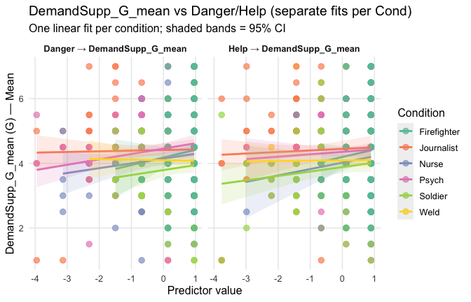
[If there were a public campaign in support of journalists, how likely would you be to do each of these things in response?] Sharing a supportive post about journalists on my social media

Toggle details of the models diagnostics and outlier analyses

Below, you’ll find model diagnostics (QQ plot, fitted vs residuals, linearity), Outliers analysis, and more details on the output

[NOTE THAT EFFECT SIZES REPORTED IN THE REPORT COMMANDS BELOW SHOULD NOT BE TRUSTED]

paste0("####################################################")

## [1] "####################################################"

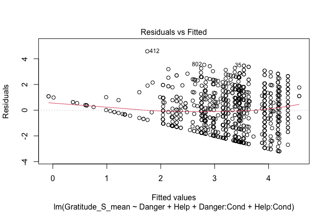
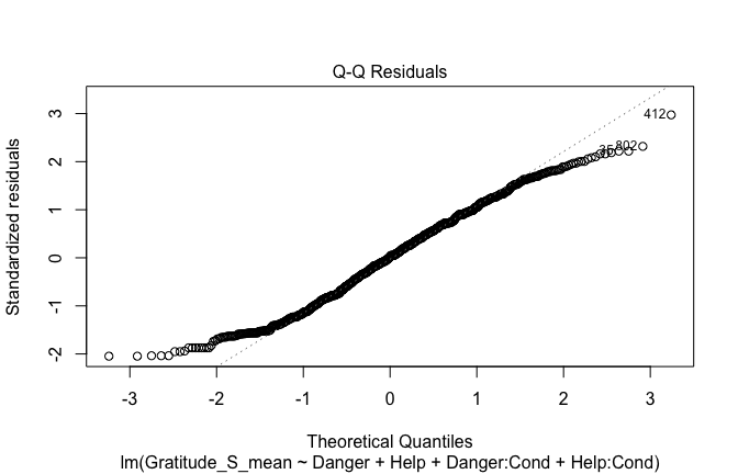
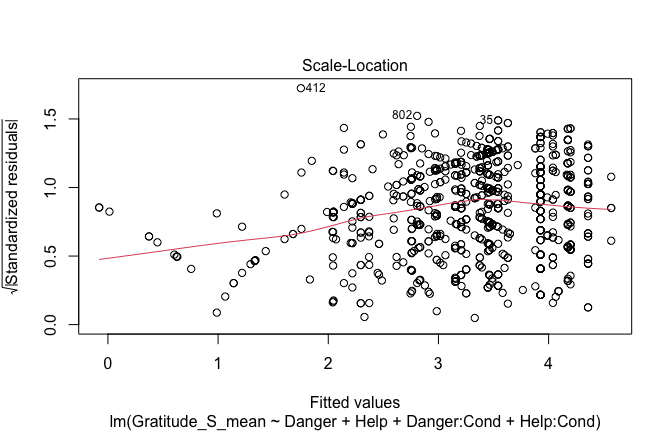
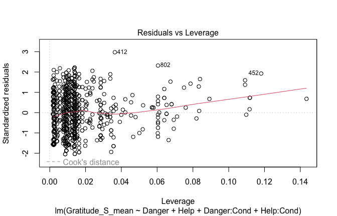
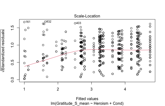
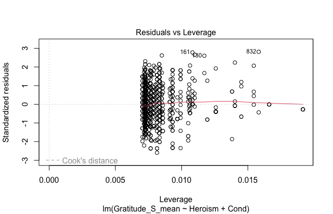
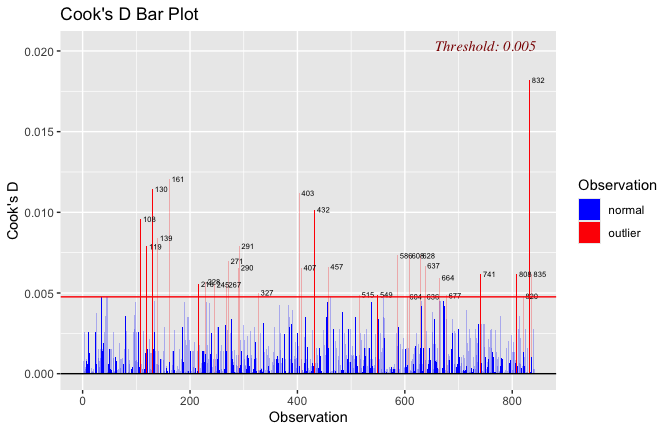
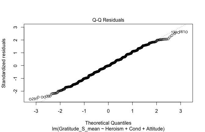
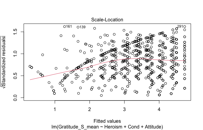
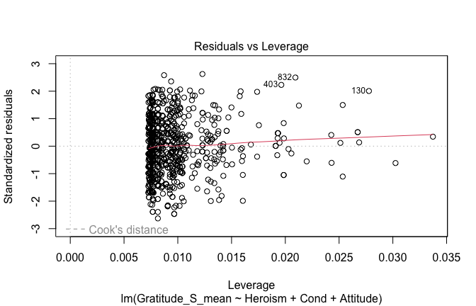
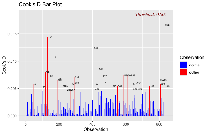
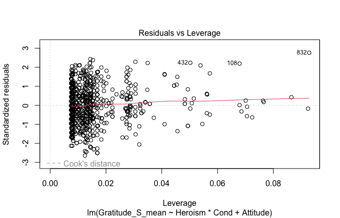
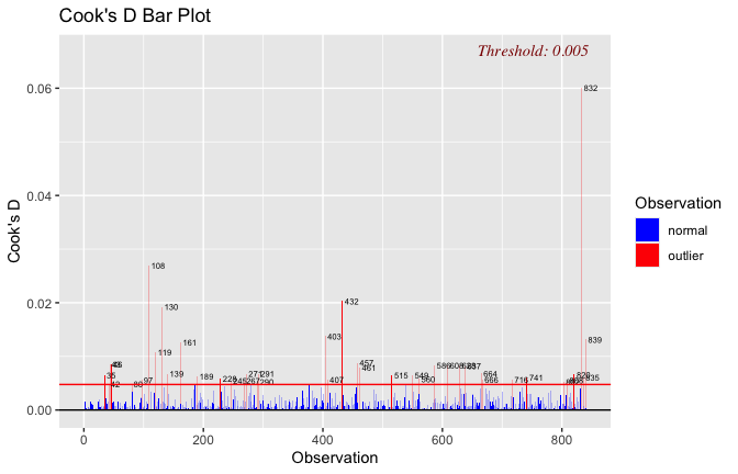
paste0("Diagnostics for Model 1: DV ~ Heroism + Occupation")

## [1] "Diagnostics for Model 1: DV ~ Heroism + Occupation"

paste0("####################################################")

## [1] "####################################################"

mod1 <- lm(Gratitude_S_mean ~ Heroism  + Cond, data = scale_scores)
mod1r <- lmrob(Gratitude_S_mean ~ Heroism  + Cond, data = scale_scores)
plot(mod1)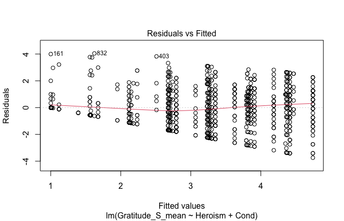

ols_plot_cooksd_bar(mod1, type = 1)

paste0("Comparison with Robust model")

## [1] "Comparison with Robust model"

models <- list("OLS (lm)" = mod1, "Robust (lmrob)" = mod1r)
modelsummary(
  models,
  statistic = c("({std.error})", "{statistic}", "p = {p.value}"),
  gof_omit  = "IC|Log.Lik",   # robust AIC comparability is iffy; omit by default
  output    = "html"
)

	OLS (lm)	Robust (lmrob)
(Intercept)	0.546	0.337
	(0.176)	(0.163)
	3.096	2.069
	p = 0.002	p = 0.039
Heroism	0.558	0.600
	(0.034)	(0.034)
	16.262	17.539
	p = <0.001	p = <0.001
Cond1	−0.039	−0.054
	(0.116)	(0.127)
	−0.337	−0.427
	p = 0.736	p = 0.670
Cond2	−0.103	−0.094
	(0.121)	(0.130)
	−0.850	−0.722
	p = 0.395	p = 0.470
Cond3	0.289	0.314
	(0.114)	(0.118)
	2.538	2.653
	p = 0.011	p = 0.008
Cond4	0.014	0.006
	(0.112)	(0.117)
	0.126	0.049
	p = 0.900	p = 0.961
Cond5	−0.089	−0.094
	(0.112)	(0.120)
	−0.795	−0.788
	p = 0.427	p = 0.431
Num.Obs.	840	840
R2	0.307	0.332
R2 Adj.	0.302	0.328
RMSE	1.44	1.44

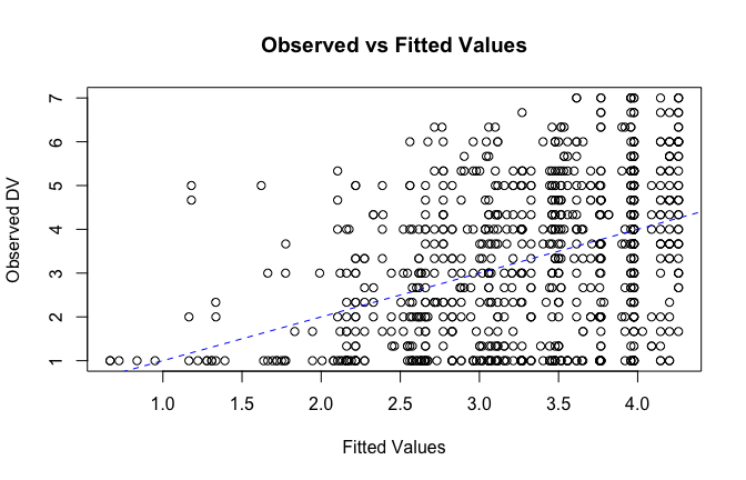
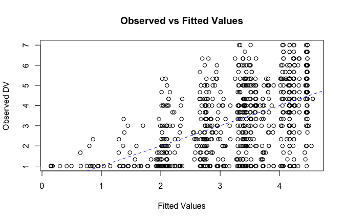
fitted_vals <- fitted(mod1)

# Plot observed values against fitted values
plot(fitted_vals, scale_scores$Gratitude_S_mean,
     xlab = "Fitted Values",
     ylab = "Observed DV",
     main = "Observed vs Fitted Values")
abline(0, 1, col = "blue", lty = 2)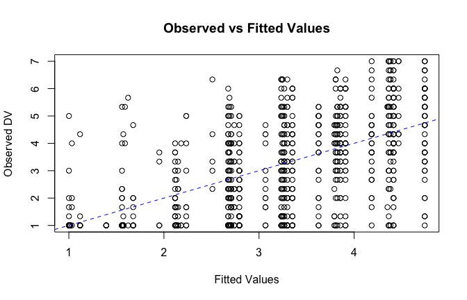

paste0("####################################################")

## [1] "####################################################"

paste0("Diagnostics for Model 2: DV ~ Heroism * Occupation")

## [1] "Diagnostics for Model 2: DV ~ Heroism * Occupation"

paste0("####################################################")

## [1] "####################################################"

mod1 <- lm(Gratitude_S_mean ~ Heroism  * Cond, data = scale_scores)
mod1r <- lmrob(Gratitude_S_mean ~ Heroism  * Cond, data = scale_scores)
plot(mod1)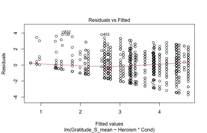

ols_plot_cooksd_bar(mod1, type = 1)

paste0("Comparison with Robust model")

## [1] "Comparison with Robust model"

models <- list("OLS (lm)" = mod1, "Robust (lmrob)" = mod1r)
modelsummary(
  models,
  statistic = c("({std.error})", "{statistic}", "p = {p.value}"),
  gof_omit  = "IC|Log.Lik",   # robust AIC comparability is iffy; omit by default
  output    = "html"
)

	OLS (lm)	Robust (lmrob)
(Intercept)	0.511	0.234
	(0.186)	(0.198)
	2.748	1.181
	p = 0.006	p = 0.238
Heroism	0.559	0.609
	(0.035)	(0.039)
	15.802	15.807
	p = <0.001	p = <0.001
Cond1	−0.098	−0.461
	(0.556)	(0.662)
	−0.176	−0.696
	p = 0.860	p = 0.486
Cond2	0.470	0.622
	(0.316)	(0.276)
	1.487	2.253
	p = 0.137	p = 0.025
Cond3	0.386	0.488
	(0.414)	(0.354)
	0.931	1.378
	p = 0.352	p = 0.168
Cond4	−0.238	−0.176
	(0.374)	(0.328)
	−0.637	−0.536
	p = 0.525	p = 0.592
Cond5	−0.399	−0.317
	(0.372)	(0.304)
	−1.071	−1.042
	p = 0.284	p = 0.298
Heroism × Cond1	0.015	0.076
	(0.093)	(0.110)
	0.165	0.689
	p = 0.869	p = 0.491
Heroism × Cond2	−0.152	−0.192
	(0.075)	(0.078)
	−2.022	−2.448
	p = 0.043	p = 0.015
Heroism × Cond3	−0.011	−0.022
	(0.072)	(0.065)
	−0.156	−0.335
	p = 0.876	p = 0.738
Heroism × Cond4	0.063	0.054
	(0.077)	(0.071)
	0.821	0.754
	p = 0.412	p = 0.451
Heroism × Cond5	0.067	0.057
	(0.070)	(0.065)
	0.964	0.878
	p = 0.335	p = 0.380
Num.Obs.	840	840
R2	0.312	0.345
R2 Adj.	0.302	0.336
RMSE	1.44	1.44

fitted_vals <- fitted(mod1)

# Plot observed values against fitted values
plot(fitted_vals, scale_scores$Gratitude_S_mean,
     xlab = "Fitted Values",
     ylab = "Observed DV",
     main = "Observed vs Fitted Values")
abline(0, 1, col = "blue", lty = 2)

paste0("####################################################")

## [1] "####################################################"

paste0("Diagnostics for Model 3: DV ~ Heroism + Occupation + Attitude")

## [1] "Diagnostics for Model 3: DV ~ Heroism + Occupation + Attitude"

paste0("####################################################")

## [1] "####################################################"

mod1 <- lm(Gratitude_S_mean ~ Heroism  + Cond + Attitude, data = scale_scores)
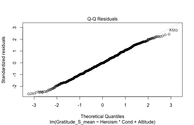
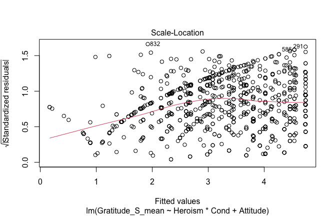
mod1r <- lmrob(Gratitude_S_mean ~ Heroism  + Cond + Attitude, data = scale_scores)
plot(mod1)

ols_plot_cooksd_bar(mod1, type = 1)

paste0("Comparison with Robust model")

## [1] "Comparison with Robust model"

models <- list("OLS (lm)" = mod1, "Robust (lmrob)" = mod1r)
modelsummary(
  models,
  statistic = c("({std.error})", "{statistic}", "p = {p.value}"),
  gof_omit  = "IC|Log.Lik",   # robust AIC comparability is iffy; omit by default
  output    = "html"
)

	OLS (lm)	Robust (lmrob)
(Intercept)	1.391	1.220
	(0.240)	(0.278)
	5.790	4.393
	p = <0.001	p = <0.001
Heroism	0.387	0.423
	(0.048)	(0.056)
	8.104	7.590
	p = <0.001	p = <0.001
Cond1	−0.126	−0.137
	(0.116)	(0.131)
	−1.082	−1.051
	p = 0.279	p = 0.293
Cond2	0.030	0.031
	(0.122)	(0.129)
	0.242	0.239
	p = 0.809	p = 0.811
Cond3	0.214	0.242
	(0.113)	(0.119)
	1.891	2.030
	p = 0.059	p = 0.043
Cond4	−0.027	−0.042
	(0.111)	(0.117)
	−0.242	−0.359
	p = 0.809	p = 0.720
Cond5	−0.018	−0.012
	(0.112)	(0.120)
	−0.164	−0.096
	p = 0.869	p = 0.923
Attitude	0.408	0.396
	(0.080)	(0.087)
	5.094	4.553
	p = <0.001	p = <0.001
Num.Obs.	840	840
R2	0.328	0.345
R2 Adj.	0.323	0.340
RMSE	1.42	1.42

fitted_vals <- fitted(mod1)

# Plot observed values against fitted values
plot(fitted_vals, scale_scores$Gratitude_S_mean,
     xlab = "Fitted Values",
     ylab = "Observed DV",
     main = "Observed vs Fitted Values")
abline(0, 1, col = "blue", lty = 2)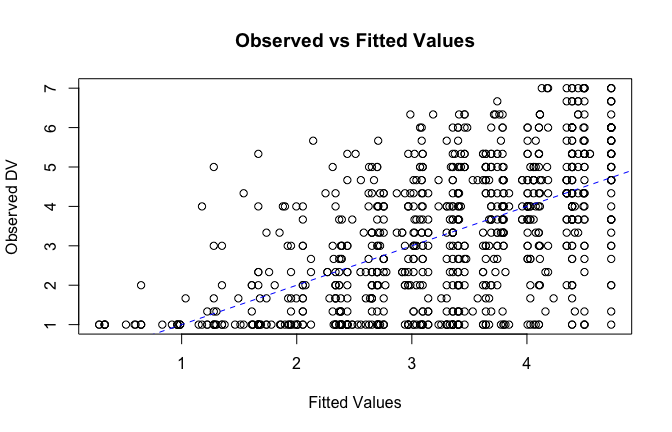

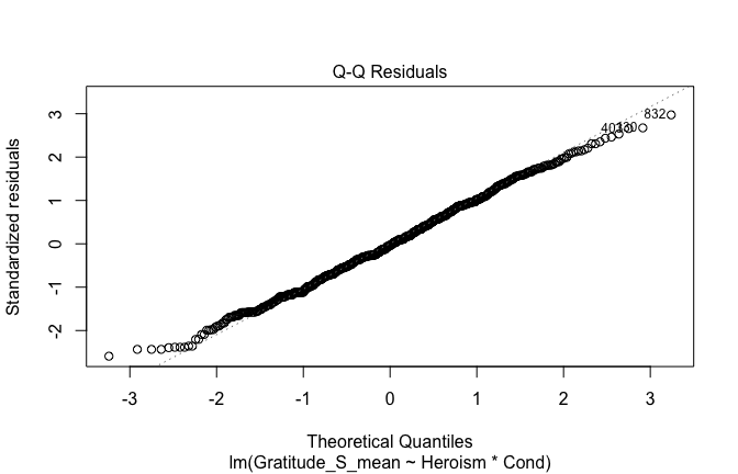
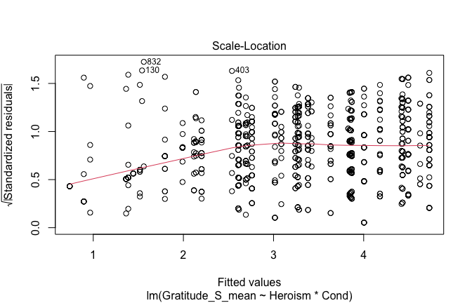
paste0("####################################################")

## [1] "####################################################"

paste0("Diagnostics for Model 4: DV ~ Heroism * Occupation + Attitude")

## [1] "Diagnostics for Model 4: DV ~ Heroism * Occupation + Attitude"

paste0("####################################################")

## [1] "####################################################"

mod1 <- lm(Gratitude_S_mean ~ Heroism*Cond + Attitude, data = scale_scores)
mod1r <- lmrob(Gratitude_S_mean ~ Heroism*Cond + Attitude, data = scale_scores)
plot(mod1)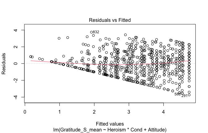

ols_plot_cooksd_bar(mod1, type = 1)

paste0("Comparison with Robust model")

## [1] "Comparison with Robust model"

models <- list("OLS (lm)" = mod1, "Robust (lmrob)" = mod1r)
modelsummary(
  models,
  statistic = c("({std.error})", "{statistic}", "p = {p.value}"),
  gof_omit  = "IC|Log.Lik",   # robust AIC comparability is iffy; omit by default
  output    = "html"
)

	OLS (lm)	Robust (lmrob)
(Intercept)	1.372	1.145
	(0.243)	(0.296)
	5.637	3.873
	p = <0.001	p = <0.001
Heroism	0.381	0.425
	(0.048)	(0.058)
	7.926	7.366
	p = <0.001	p = <0.001
Cond1	−0.443	−0.761
	(0.551)	(0.668)
	−0.805	−1.139
	p = 0.421	p = 0.255
Cond2	0.813	0.893
	(0.318)	(0.274)
	2.559	3.261
	p = 0.011	p = 0.001
Cond3	0.260	0.374
	(0.408)	(0.369)
	0.636	1.013
	p = 0.525	p = 0.311
Cond4	−0.380	−0.332
	(0.368)	(0.331)
	−1.032	−1.002
	p = 0.302	p = 0.317
Cond5	−0.005	0.037
	(0.373)	(0.315)
	−0.012	0.116
	p = 0.990	p = 0.908
Attitude	0.439	0.423
	(0.082)	(0.087)
	5.365	4.854
	p = <0.001	p = <0.001
Heroism × Cond1	0.059	0.112
	(0.092)	(0.110)
	0.643	1.014
	p = 0.521	p = 0.311
Heroism × Cond2	−0.201	−0.226
	(0.074)	(0.076)
	−2.699	−2.957
	p = 0.007	p = 0.003
Heroism × Cond3	−0.001	−0.014
	(0.071)	(0.066)
	−0.018	−0.208
	p = 0.985	p = 0.835
Heroism × Cond4	0.089	0.081
	(0.076)	(0.072)
	1.175	1.130
	p = 0.240	p = 0.259
Heroism × Cond5	0.008	0.005
	(0.070)	(0.066)
	0.112	0.081
	p = 0.911	p = 0.935
Num.Obs.	840	840
R2	0.335	0.358
R2 Adj.	0.325	0.348
RMSE	1.41	1.41

fitted_vals <- fitted(mod1)

# Plot observed values against fitted values
plot(fitted_vals, scale_scores$Gratitude_S_mean,
     xlab = "Fitted Values",
     ylab = "Observed DV",
     main = "Observed vs Fitted Values")
abline(0, 1, col = "blue", lty = 2)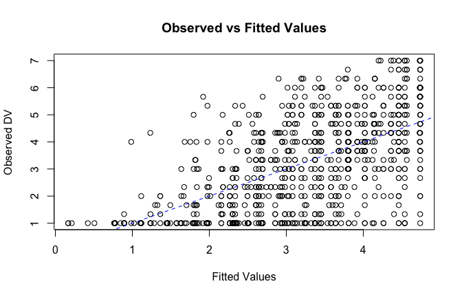

paste0("####################################################")

## [1] "####################################################"

paste0("REPORTS for each model (please ignore the eta squares, they are way off")

## [1] "REPORTS for each model (please ignore the eta squares, they are way off"

paste0("####################################################")

## [1] "####################################################"

paste0("MODEL 1: Gratitude_S_mean ~ Heroism")

## [1] "MODEL 1: Gratitude_S_mean ~ Heroism"

report(Anova(mod1 <- lm(Gratitude_S_mean ~ Heroism  + Cond, data = scale_scores), type = "III"))

## The ANOVA suggests that:
## 
##   - The main effect of Heroism is statistically significant and large (F(1, 833)
## = 264.46, p < .001; Eta2 (partial) = 0.24, 95% CI [0.20, 1.00])
##   - The main effect of Cond is statistically not significant and very small (F(5,
## 833) = 1.39, p = 0.224; Eta2 (partial) = 8.30e-03, 95% CI [0.00, 1.00])
## 
## Effect sizes were labelled following Field's (2013) recommendations.

paste0("MODEL 2: Gratitude_S_mean ~ Heroism * Cond")

## [1] "MODEL 2: Gratitude_S_mean ~ Heroism * Cond"

report(Anova(mod2 <- lm(Gratitude_S_mean ~ Heroism * Cond, data = scale_scores), type = "III"))

## Type 3 ANOVAs only give sensible and informative results when covariates
##   are mean-centered and factors are coded with orthogonal contrasts (such
##   as those produced by `contr.sum`, `contr.poly`, or `contr.helmert`, but
##   *not* by the default `contr.treatment`).

## The ANOVA suggests that:
## 
##   - The main effect of Heroism is statistically significant and large (F(1, 828)
## = 249.71, p < .001; Eta2 (partial) = 0.23, 95% CI [0.19, 1.00])
##   - The main effect of Cond is statistically not significant and very small (F(5,
## 828) = 0.87, p = 0.500; Eta2 (partial) = 5.23e-03, 95% CI [0.00, 1.00])
##   - The interaction between Heroism and Cond is statistically not significant and
## very small (F(5, 828) = 1.00, p = 0.419; Eta2 (partial) = 5.98e-03, 95% CI
## [0.00, 1.00])
## 
## Effect sizes were labelled following Field's (2013) recommendations.

paste0("MODEL 3: Gratitude_S_mean ~ Heroism +scale(Attitude)")

## [1] "MODEL 3: Gratitude_S_mean ~ Heroism +scale(Attitude)"

report(Anova(mod3 <- lm(Gratitude_S_mean ~ Heroism   + Cond +scale(Attitude) , data = scale_scores), type = "III"))

## The ANOVA suggests that:
## 
##   - The main effect of Heroism is statistically significant and medium (F(1, 832)
## = 65.67, p < .001; Eta2 (partial) = 0.07, 95% CI [0.05, 1.00])
##   - The main effect of Cond is statistically not significant and very small (F(5,
## 832) = 0.95, p = 0.445; Eta2 (partial) = 5.70e-03, 95% CI [0.00, 1.00])
##   - The main effect of scale(Attitude) is statistically significant and small
## (F(1, 832) = 25.95, p < .001; Eta2 (partial) = 0.03, 95% CI [0.01, 1.00])
## 
## Effect sizes were labelled following Field's (2013) recommendations.

paste0("MODEL 4: Gratitude_S_mean ~ Heroism * Cond + scale(Attitude)")

## [1] "MODEL 4: Gratitude_S_mean ~ Heroism * Cond + scale(Attitude)"

report(Anova(mod4 <-lm(Gratitude_S_mean ~ Heroism * Cond + scale(Attitude), data = scale_scores), type = "III"))

## Type 3 ANOVAs only give sensible and informative results when covariates
##   are mean-centered and factors are coded with orthogonal contrasts (such
##   as those produced by `contr.sum`, `contr.poly`, or `contr.helmert`, but
##   *not* by the default `contr.treatment`).

## The ANOVA suggests that:
## 
##   - The main effect of Heroism is statistically significant and medium (F(1, 827)
## = 62.81, p < .001; Eta2 (partial) = 0.07, 95% CI [0.05, 1.00])
##   - The main effect of Cond is statistically not significant and very small (F(5,
## 827) = 1.60, p = 0.158; Eta2 (partial) = 9.56e-03, 95% CI [0.00, 1.00])
##   - The main effect of scale(Attitude) is statistically significant and small
## (F(1, 827) = 28.78, p < .001; Eta2 (partial) = 0.03, 95% CI [0.02, 1.00])
##   - The interaction between Heroism and Cond is statistically not significant and
## very small (F(5, 827) = 1.58, p = 0.163; Eta2 (partial) = 9.46e-03, 95% CI
## [0.00, 1.00])
## 
## Effect sizes were labelled following Field's (2013) recommendations.

paste0("Model Comparison: assessing the importance of attitude - not accounting for occupations")

## [1] "Model Comparison: assessing the importance of attitude - not accounting for occupations"

anova(mod1, mod3)

paste0("Model Comparison: assessing the importance of attitude - accounting for occupations")

## [1] "Model Comparison: assessing the importance of attitude - accounting for occupations"

anova(mod2, mod4)

ggplot(scale_scores, aes(y = Gratitude_S_mean, x = Heroism)) +
  # 1) points colored by Cond
  geom_point(aes(color = Cond),
             size = 2.7, alpha = 0.7) +
  
  # 2) ONE global lm line (group = 1 prevents one line per Cond)
  stat_smooth(method = "lm", se = TRUE,
              aes(group = 1),
              color = "black", linewidth = 1) +
  
  # Nice, accessible palette (works well with >3 groups)
  scale_color_brewer(palette = "Set2") +
  
  labs(
    y = "Gratitude (S)",
    x = "Heroism",
    color = "Occupation",
    title = "Heroism vs. Gratitude (S), colored by Occupation",
    subtitle = "Points are participants; black line is overall linear fit with 95% CI"
  ) +
  theme_minimal(base_size = 12) +
  theme(
    legend.position = "right",
    panel.grid.minor = element_blank()
  )

## `geom_smooth()` using formula = 'y ~ x'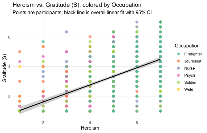

ggplot(scale_scores, aes(y = Gratitude_S_mean, x = Heroism, color = Cond)) +
  # points colored by condition
  geom_point(size = 2.7, alpha = 0.7) +
  # ONE lm line PER condition (because color is mapped here)
  stat_smooth(method = "lm", se = FALSE, linewidth = 1, fullrange = TRUE) +
  scale_color_brewer(palette = "Set2") +
  labs(
    y = "Gratitude (S)",
    x = "Heroism",
    color = "Occupation",
    title = "Heroism vs. Gratitude (S) with per-Occupation linear fits"
  ) +
  theme_minimal(base_size = 12) +
  theme(legend.position = "right", panel.grid.minor = element_blank())

## `geom_smooth()` using formula = 'y ~ x'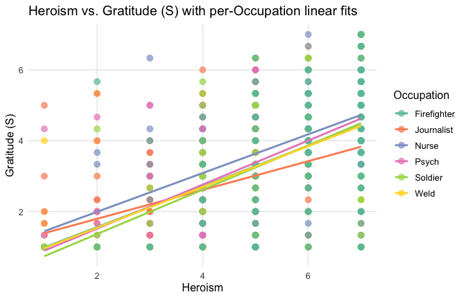

Overall: Heroism predict specific gratitude. This is true above and beyond attitude (see Model 3). It is true when controlling for normative effects of occupations (Model 2), and when controlling for both occupations and attitude (Model 4). See Summary table:

Model 1: “~Heroism + Occupation”

# =========================
# OLD MODELS (Heroism)
# =========================
m1_H <- lm(Gratitude_S_mean ~ Heroism + Occupation, data = scale_scores)
m2_H <- lm(Gratitude_S_mean ~ Heroism * Occupation, data = scale_scores)
m3_H <- lm(Gratitude_S_mean ~ Heroism + Occupation + Attitude, data = scale_scores)
m4_H <- lm(Gratitude_S_mean ~ Heroism * Occupation + Attitude, data = scale_scores)

tidy_type3(m1_H, "~Heroism + Cond")

~Heroism + Cond
	Term	df1	df2	F	p	eta2p
Heroism	Heroism	1	833	264.46	< .001	0.241
Occupation	Occupation	5	833	1.39	= 0.224	0.008

# =========================
# NEW MODELS (Danger & Help)
# =========================

Model 2: “~Heroism * Occupation”

tidy_type3(m2_H, "~Heroism * Cond")

~Heroism * Cond
	Term	df1	df2	F	p	eta2p
Heroism	Heroism	1	828	249.71	< .001	0.232
Occupation	Occupation	5	828	0.87	= 0.500	0.005
Heroism:Occupation	Heroism:Occupation	5	828	1.00	= 0.419	0.006

Model 3: “~Heroism + Occupation + Attitude”

tidy_type3(m3_H, "~Heroism + Occupation + Attitude")

~Heroism + Occupation + Attitude
	Term	df1	df2	F	p	eta2p
Heroism	Heroism	1	832	65.67	< .001	0.073
Occupation	Occupation	5	832	0.95	= 0.445	0.006
Attitude	Attitude	1	832	25.95	< .001	0.030

Model 4: “~Heroism * Occupation + Attitude”

tidy_type3(m4_H, "~Heroism * Occupation + Attitude")

~Heroism * Occupation + Attitude
	Term	df1	df2	F	p	eta2p
Heroism	Heroism	1	827	62.81	< .001	0.071
Occupation	Occupation	5	827	1.60	= 0.158	0.010
Attitude	Attitude	1	827	28.78	< .001	0.034
Heroism:Occupation	Heroism:Occupation	5	827	1.58	= 0.163	0.009

==> Full support for our hypotheses. Across all occupations Heroism predict general- and specific-level gratitude, with or without controlling for attitude.

Comparison of main effects across models

# Use orthogonal contrasts; keeps your "Heroism main effect" interpretable with Cond in the model
old_contr <- options(contrasts = c("contr.sum", "contr.poly"))

# Helper to extract the main effect of "Heroism" from a car::Anova table
extract_heroism <- function(mod, model_label) {
  a <- car::Anova(mod, type = "III")

  # Coerce to data.frame with rownames preserved
  tab <- as.data.frame(a)
  tab$Term <- rownames(tab)

  # Standard column names across R versions
  # (car::Anova uses these names for lm/glm type=III)
  # Columns: "Sum Sq", "Df", "F value", "Pr(>F)"
  names(tab) <- sub(" ", "_", names(tab))  # make names safe: "Sum_Sq", "F_value", etc.

  # Pull rows we need
  hero <- tab %>% filter(Term == "Heroism")
  resid <- tab %>% filter(Term == "Residuals")

  # Safety checks (in case of name variants)
  stopifnot(nrow(hero) == 1, nrow(resid) == 1)

  # Partial eta^2 = SS_effect / (SS_effect + SS_residual)
  eta_p2 <- hero$Sum_Sq / (hero$Sum_Sq + resid$Sum_Sq)

  # Format p nicely (APA-ish)
  p_fmt <- ifelse(hero$`Pr(>F)` < .001, "< .001",
                  sprintf("= %.3f", hero$`Pr(>F)`))

  dplyr::tibble(
    Model = model_label,
    Outcome = "Gratitude_S_mean",
    Predictor = "Heroism",
    df1 = hero$Df,
    df2 = resid$Df,
    F = hero$F_value,
    p = p_fmt,
    eta2p = eta_p2
  )
}

# ----- Fit the four models -----
mod1 <- lm(Gratitude_S_mean ~ Heroism   + Cond, data = scale_scores)
mod2 <- lm(Gratitude_S_mean ~ Heroism * Cond, data = scale_scores)
mod3 <- lm(Gratitude_S_mean ~ Heroism   + Cond + scale(Attitude), data = scale_scores)
mod4 <- lm(Gratitude_S_mean ~ Heroism * Cond + scale(Attitude), data = scale_scores)

# ----- Build the summary table -----
tbl <- bind_rows(
  extract_heroism(mod1, "~ Heroism   + Cond"),
  extract_heroism(mod2, "~ Heroism * Occupation"),
  extract_heroism(mod3, "~ Heroism   + Cond + Attitude"),
  extract_heroism(mod4, "~ Heroism * Occupation + Attitude")
  ) %>%
  # Nice number formatting for F and eta^2p
  mutate(
    F = round(F, 2),
    eta2p = round(eta2p, 3)
  )

# ----- Print as HTML-friendly table -----
# Build the table first
tbl_kbl <- tbl %>%
  kable("html",
        caption = "Main effect of Heroism across models (Type-III ANOVA): F, p, partial η²",
        align = "lllrrrcr")
# Add a footnote in a version-robust way
if ("footnote" %in% getNamespaceExports("kableExtra")) {
  tbl_kbl <- tbl_kbl %>%
    kableExtra::footnote(
      general = "Type-III sums of squares with sum contrasts. Partial η² = SS_effect / (SS_effect + SS_residual). p values are APA-style.",
      general_title = ""
    )
} else {
  tbl_kbl <- tbl_kbl %>%
    kableExtra::add_footnote(
      label = "Type-III sums of squares with sum contrasts. Partial η² = SS_effect / (SS_effect + SS_residual). p values are APA-style.",
      notation = "none"
    )
}

tbl_kbl

Main effect of Heroism across models (Type-III ANOVA): F, p, partial η²
Model	Outcome	Predictor	df1	df2	F	p	eta2p
~ Heroism + Cond	Gratitude_S_mean	Heroism	1	833	264.46	< .001	0.241
~ Heroism * Occupation	Gratitude_S_mean	Heroism	1	828	249.71	< .001	0.232
~ Heroism + Cond + Attitude	Gratitude_S_mean	Heroism	1	832	65.67	< .001	0.073
~ Heroism * Occupation + Attitude	Gratitude_S_mean	Heroism	1	827	62.81	< .001	0.071
Type-III sums of squares with sum contrasts. Partial η² = SS_effect / (SS_effect + SS_residual). p values are APA-style.

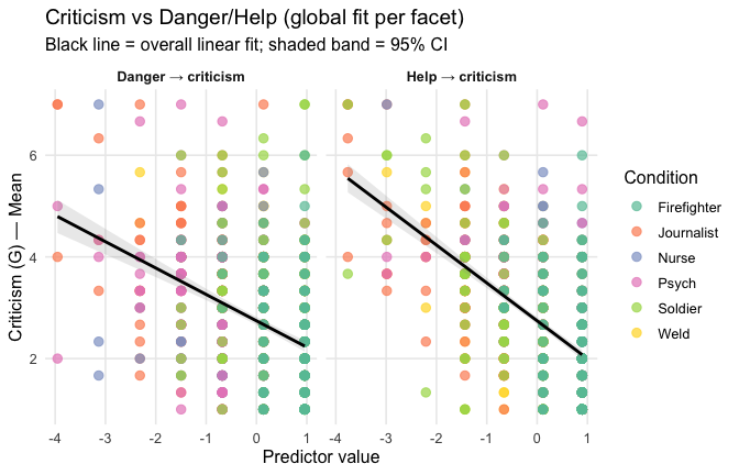
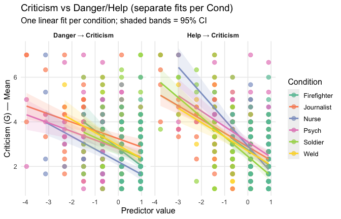
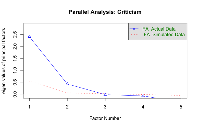
H2: Heroism is associated with reduced criticism acceptability

Criticism of those granted moral goodness through the ‘hero’ status might be seen as a violation of sacred values (Tetlock, 2003). As such, people should report that people should not criticise the heroised workers at the general level. At the specific level, they should be more likely to approve for prosecutions and bans imposed to people who openly criticised the target workers.

General level

People should think twice before they criticize journalists

Toggle details of the models diagnostics and outlier analyses

Below, you’ll find model diagnostics (QQ plot, fitted vs residuals, linearity), Outliers analysis, and more details on the output

[NOTE THAT EFFECT SIZES REPORTED IN THE REPORT COMMANDS BELOW SHOULD NOT BE TRUSTED]

paste0("####################################################")

## [1] "####################################################"

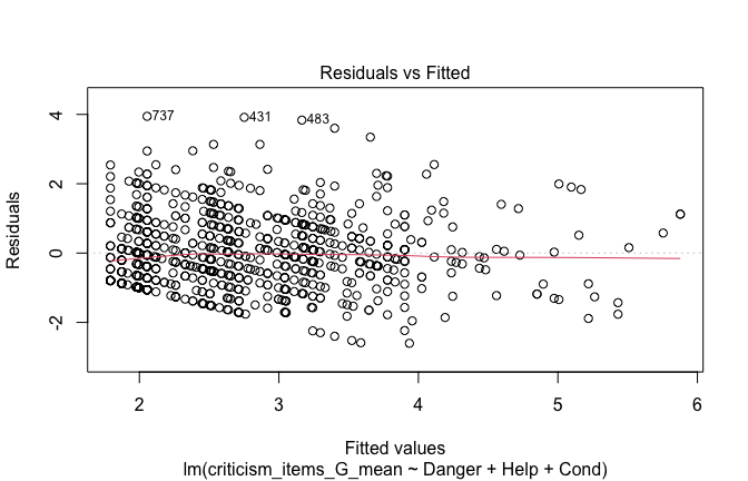
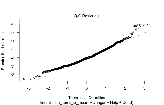
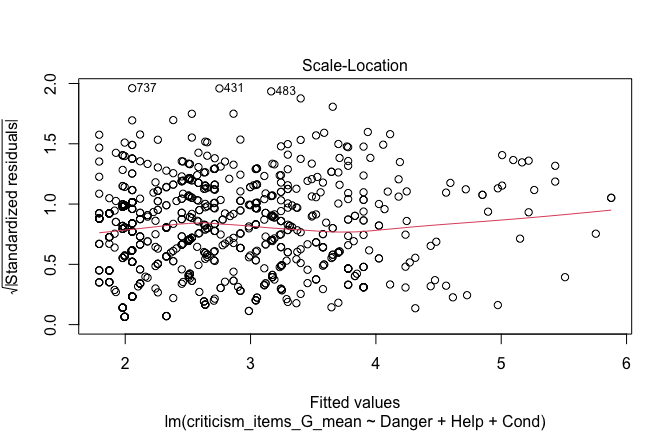
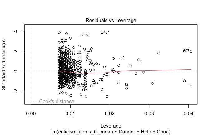
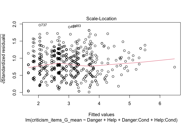
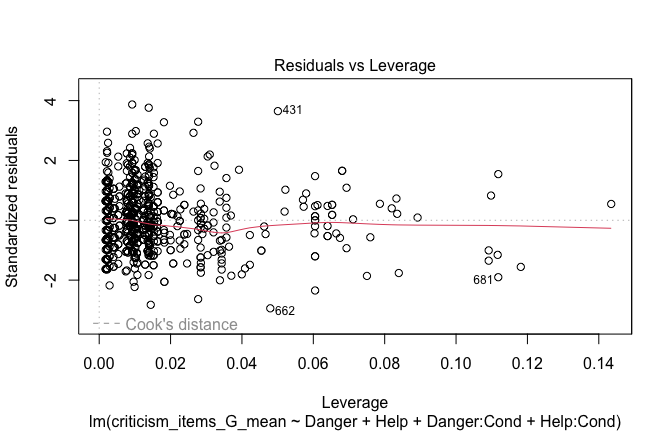
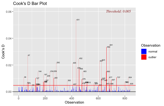
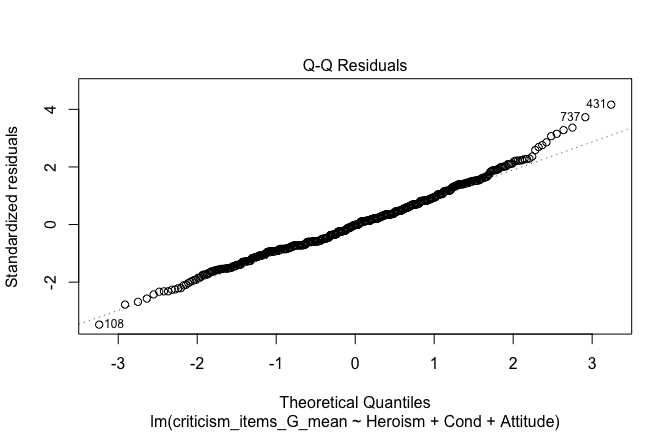
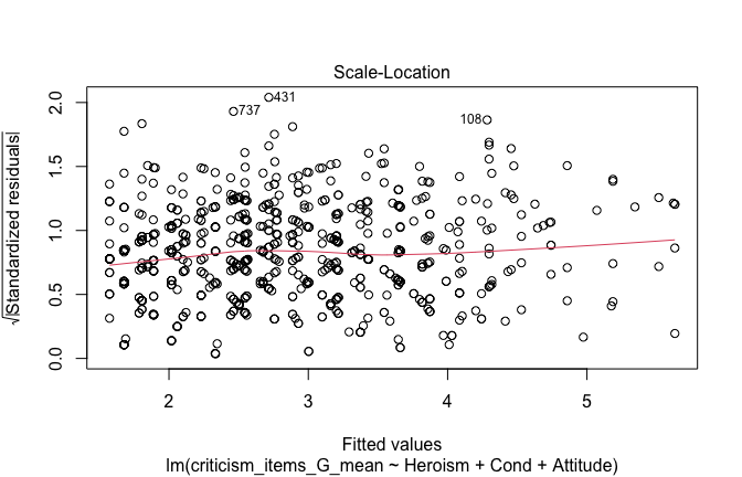
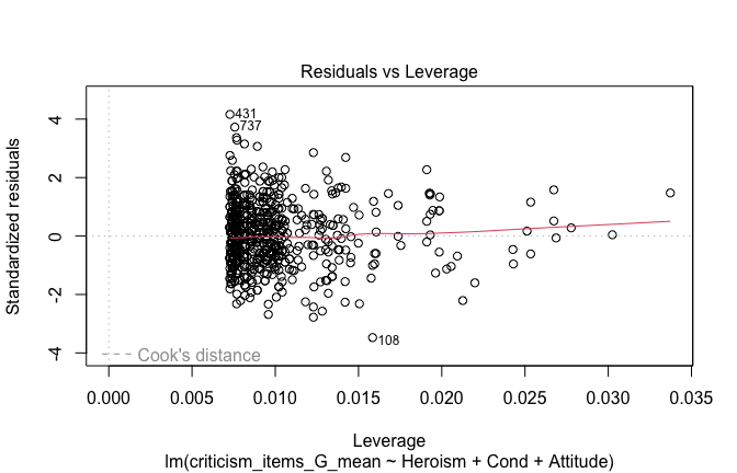
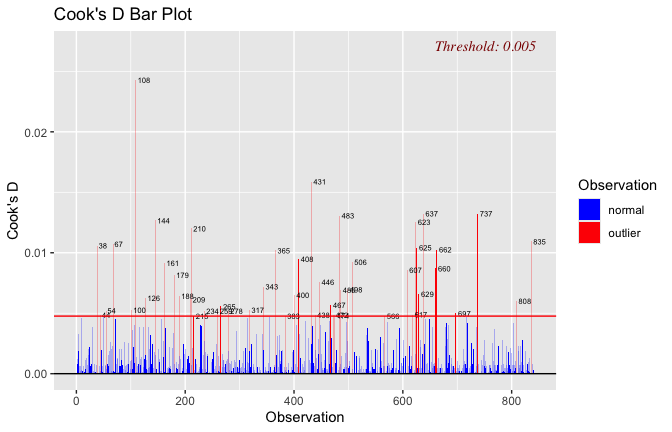
paste0("Diagnostics for Model 1: DV ~ Heroism + Occupation")

## [1] "Diagnostics for Model 1: DV ~ Heroism + Occupation"

paste0("####################################################")

## [1] "####################################################"

mod1 <- lm(criticism_items_G_mean ~ Heroism  + Cond, data = scale_scores)
mod1r <- lmrob(criticism_items_G_mean ~ Heroism  + Cond, data = scale_scores)
plot(mod1)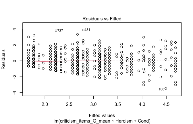

ols_plot_cooksd_bar(mod1, type = 1)

paste0("Comparison with Robust model")

## [1] "Comparison with Robust model"

models <- list("OLS (lm)" = mod1, "Robust (lmrob)" = mod1r)
modelsummary(
  models,
  statistic = c("({std.error})", "{statistic}", "p = {p.value}"),
  gof_omit  = "IC|Log.Lik",   # robust AIC comparability is iffy; omit by default
  output    = "html"
)

	OLS (lm)	Robust (lmrob)
(Intercept)	4.979	5.045
	(0.124)	(0.172)
	40.247	29.258
	p = <0.001	p = <0.001
Heroism	−0.454	−0.473
	(0.024)	(0.032)
	−18.840	−14.819
	p = <0.001	p = <0.001
Cond1	−0.027	−0.039
	(0.082)	(0.072)
	−0.328	−0.542
	p = 0.743	p = 0.588
Cond2	0.164	0.171
	(0.085)	(0.094)
	1.932	1.823
	p = 0.054	p = 0.069
Cond3	−0.139	−0.136
	(0.080)	(0.079)
	−1.742	−1.734
	p = 0.082	p = 0.083
Cond4	0.078	0.072
	(0.079)	(0.082)
	0.989	0.873
	p = 0.323	p = 0.383
Cond5	−0.038	−0.042
	(0.079)	(0.085)
	−0.482	−0.489
	p = 0.630	p = 0.625
Num.Obs.	840	840
R2	0.381	0.411
R2 Adj.	0.376	0.407
RMSE	1.01	1.01

fitted_vals <- fitted(mod1)

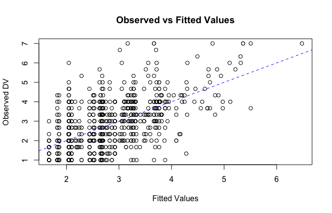
# Plot observed values against fitted values
plot(fitted_vals, scale_scores$criticism_items_G_mean,
     xlab = "Fitted Values",
     ylab = "Observed DV",
     main = "Observed vs Fitted Values")
abline(0, 1, col = "blue", lty = 2)

paste0("####################################################")

## [1] "####################################################"

paste0("Diagnostics for Model 2: DV ~ Heroism * Occupation")

## [1] "Diagnostics for Model 2: DV ~ Heroism * Occupation"

paste0("####################################################")

## [1] "####################################################"

mod1 <- lm(criticism_items_G_mean ~ Heroism  * Cond, data = scale_scores)
mod1r <- lmrob(criticism_items_G_mean ~ Heroism  * Cond, data = scale_scores)
plot(mod1)

ols_plot_cooksd_bar(mod1, type = 1)

paste0("Comparison with Robust model")

## [1] "Comparison with Robust model"

models <- list("OLS (lm)" = mod1, "Robust (lmrob)" = mod1r)
modelsummary(
  models,
  statistic = c("({std.error})", "{statistic}", "p = {p.value}"),
  gof_omit  = "IC|Log.Lik",   # robust AIC comparability is iffy; omit by default
  output    = "html"
)

	OLS (lm)	Robust (lmrob)
(Intercept)	4.976	5.087
	(0.130)	(0.163)
	38.136	31.248
	p = <0.001	p = <0.001
Heroism	−0.449	−0.474
	(0.025)	(0.030)
	−18.115	−15.937
	p = <0.001	p = <0.001
Cond1	0.152	0.244
	(0.390)	(0.359)
	0.390	0.680
	p = 0.696	p = 0.497
Cond2	0.011	−0.200
	(0.222)	(0.289)
	0.048	−0.690
	p = 0.962	p = 0.490
Cond3	−0.148	−0.245
	(0.290)	(0.449)
	−0.511	−0.546
	p = 0.610	p = 0.585
Cond4	−0.077	−0.177
	(0.262)	(0.328)
	−0.294	−0.540
	p = 0.769	p = 0.589
Cond5	0.471	0.691
	(0.261)	(0.387)
	1.806	1.785
	p = 0.071	p = 0.075
Heroism × Cond1	−0.034	−0.054
	(0.066)	(0.059)
	−0.526	−0.917
	p = 0.599	p = 0.359
Heroism × Cond2	0.039	0.090
	(0.053)	(0.068)
	0.743	1.322
	p = 0.458	p = 0.186
Heroism × Cond3	−0.003	0.012
	(0.051)	(0.072)
	−0.054	0.160
	p = 0.957	p = 0.873
Heroism × Cond4	0.030	0.046
	(0.054)	(0.066)
	0.558	0.699
	p = 0.577	p = 0.485
Heroism × Cond5	−0.105	−0.144
	(0.049)	(0.067)
	−2.135	−2.134
	p = 0.033	p = 0.033
Num.Obs.	840	840
R2	0.385	0.429
R2 Adj.	0.377	0.421
RMSE	1.01	1.01

fitted_vals <- fitted(mod1)

# Plot observed values against fitted values
plot(fitted_vals, scale_scores$criticism_items_G_mean,
     xlab = "Fitted Values",
     ylab = "Observed DV",
     main = "Observed vs Fitted Values")
abline(0, 1, col = "blue", lty = 2)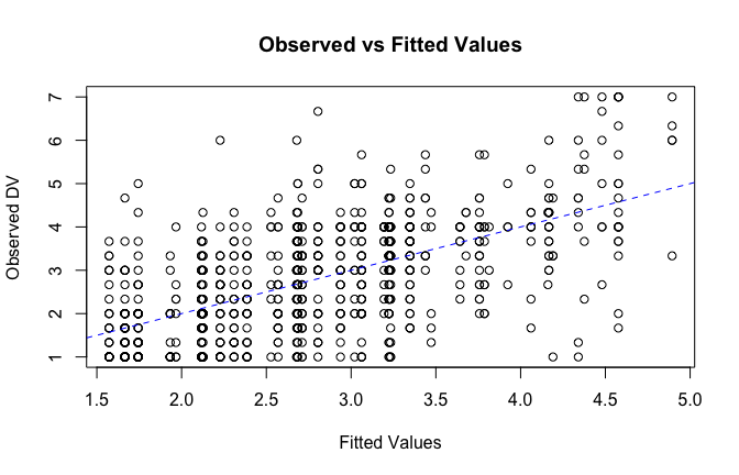

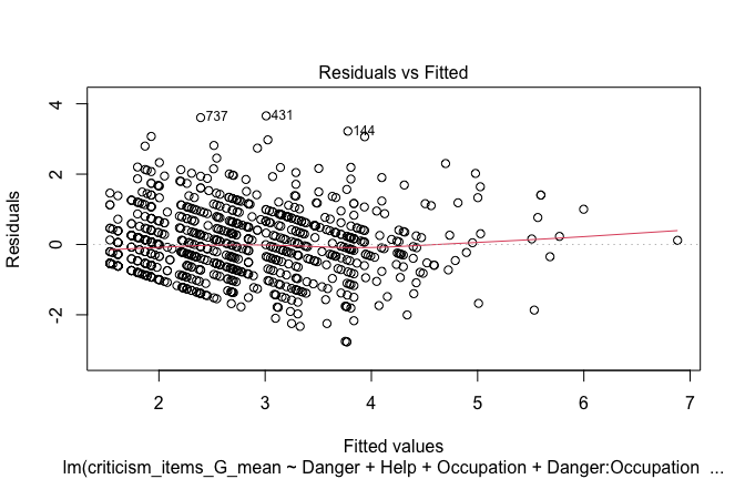
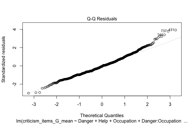
paste0("####################################################")

## [1] "####################################################"

paste0("Diagnostics for Model 3: DV ~ Heroism + Occupation + Attitude")

## [1] "Diagnostics for Model 3: DV ~ Heroism + Occupation + Attitude"

paste0("####################################################")

## [1] "####################################################"

mod1 <- lm(criticism_items_G_mean ~ Heroism  + Cond + Attitude, data = scale_scores)
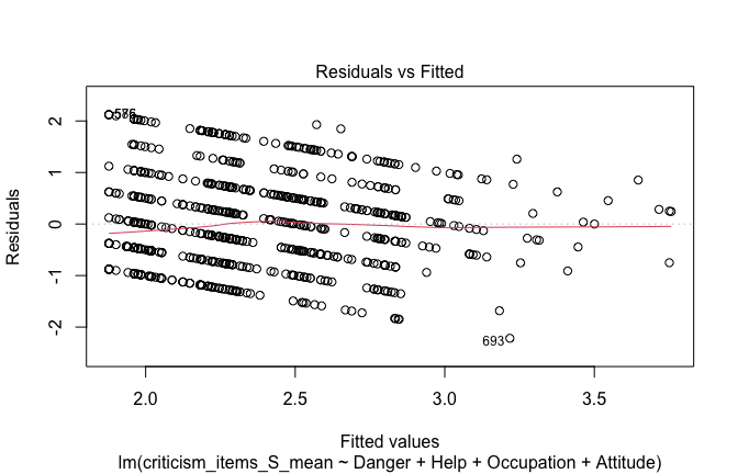
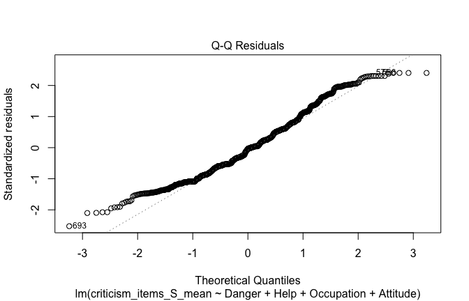
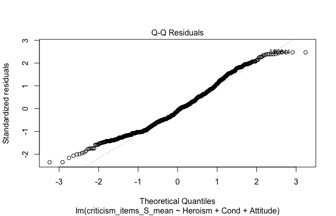
mod1r <- lmrob(criticism_items_G_mean ~ Heroism  + Cond + Attitude, data = scale_scores)
plot(mod1)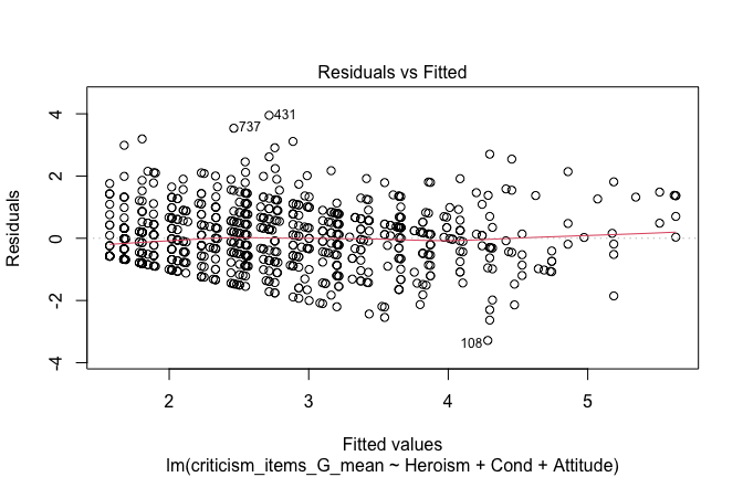

ols_plot_cooksd_bar(mod1, type = 1)

paste0("Comparison with Robust model")

## [1] "Comparison with Robust model"

models <- list("OLS (lm)" = mod1, "Robust (lmrob)" = mod1r)
modelsummary(
  models,
  statistic = c("({std.error})", "{statistic}", "p = {p.value}"),
  gof_omit  = "IC|Log.Lik",   # robust AIC comparability is iffy; omit by default
  output    = "html"
)

	OLS (lm)	Robust (lmrob)
(Intercept)	3.789	3.855
	(0.160)	(0.181)
	23.612	21.314
	p = <0.001	p = <0.001
Heroism	−0.213	−0.232
	(0.032)	(0.035)
	−6.668	−6.565
	p = <0.001	p = <0.001
Cond1	0.095	0.088
	(0.077)	(0.072)
	1.222	1.228
	p = 0.222	p = 0.220
Cond2	−0.022	−0.030
	(0.082)	(0.087)
	−0.274	−0.341
	p = 0.784	p = 0.733
Cond3	−0.034	−0.036
	(0.076)	(0.071)
	−0.445	−0.516
	p = 0.656	p = 0.606
Cond4	0.136	0.123
	(0.074)	(0.076)
	1.830	1.621
	p = 0.068	p = 0.105
Cond5	−0.138	−0.126
	(0.075)	(0.074)
	−1.849	−1.696
	p = 0.065	p = 0.090
Attitude	−0.574	−0.585
	(0.053)	(0.059)
	−10.731	−9.984
	p = <0.001	p = <0.001
Num.Obs.	840	840
R2	0.456	0.497
R2 Adj.	0.451	0.492
RMSE	0.95	0.95

fitted_vals <- fitted(mod1)

# Plot observed values against fitted values
plot(fitted_vals, scale_scores$criticism_items_G_mean,
     xlab = "Fitted Values",
     ylab = "Observed DV",
     main = "Observed vs Fitted Values")
abline(0, 1, col = "blue", lty = 2)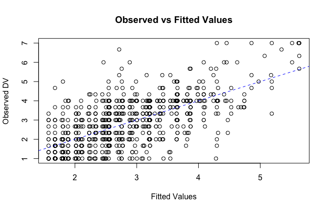

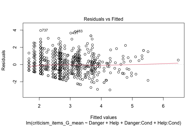
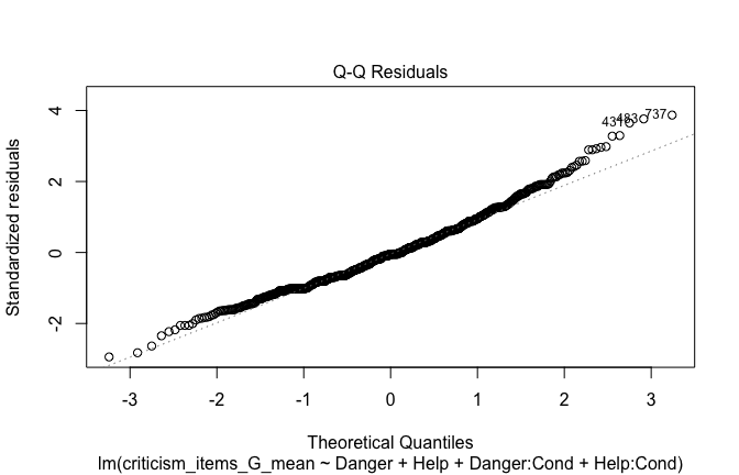
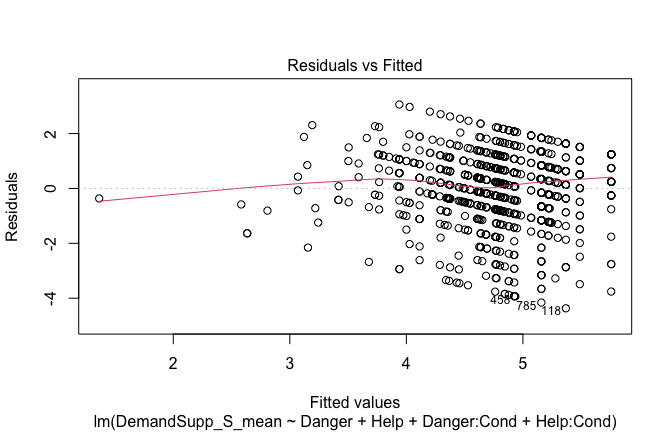
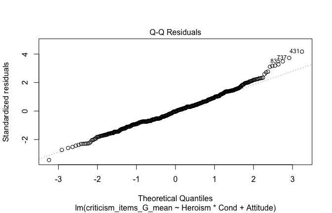
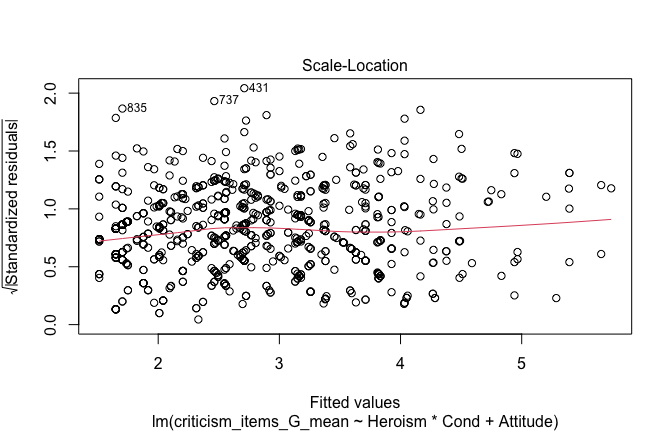
paste0("####################################################")

## [1] "####################################################"

paste0("Diagnostics for Model 4: DV ~ Heroism * Occupation + Attitude")

## [1] "Diagnostics for Model 4: DV ~ Heroism * Occupation + Attitude"

paste0("####################################################")

## [1] "####################################################"

mod1 <- lm(criticism_items_G_mean ~ Heroism*Cond + Attitude, data = scale_scores)
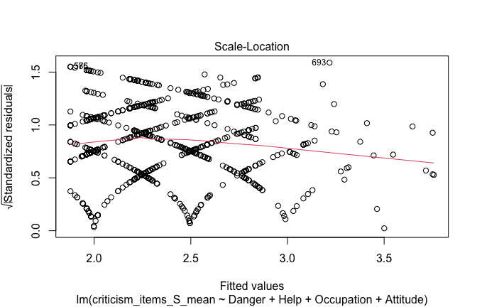
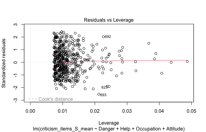
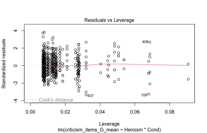
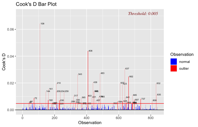
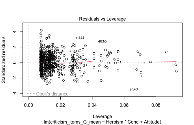
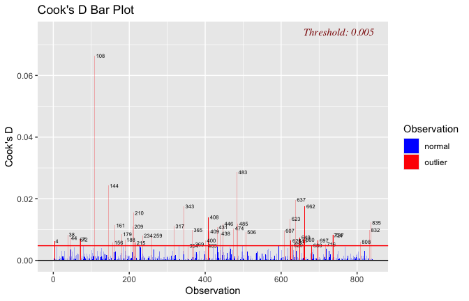
mod1r <- lmrob(criticism_items_G_mean ~ Heroism*Cond + Attitude, data = scale_scores)

## Warning in lmrob.S(x, y, control = control): S refinements did not converge (to
## refine.tol=1e-07) in 200 (= k.max) steps
## Warning in lmrob.S(x, y, control = control): S refinements did not converge (to
## refine.tol=1e-07) in 200 (= k.max) steps

## Warning in lmrob.fit(x, y, control, init = init): initial estim. 'init' not
## converged -- will be return()ed basically unchanged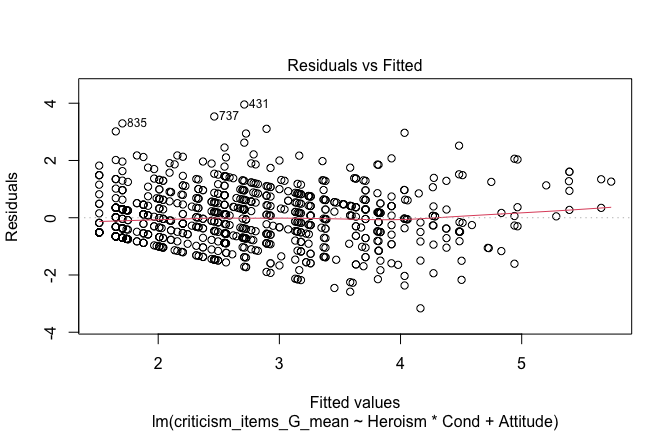

plot(mod1)

ols_plot_cooksd_bar(mod1, type = 1)

paste0("Comparison with Robust model")

## [1] "Comparison with Robust model"

models <- list("OLS (lm)" = mod1, "Robust (lmrob)" = mod1r)
modelsummary(
  models,
  statistic = c("({std.error})", "{statistic}", "p = {p.value}"),
  gof_omit  = "IC|Log.Lik",   # robust AIC comparability is iffy; omit by default
  output    = "html"
)

	OLS (lm)	Robust (lmrob)
(Intercept)	3.828	4.385
	(0.163)
	23.526
	p = <0.001
Heroism	−0.212	−0.324
	(0.032)
	−6.598
	p = <0.001
Cond1	0.612	0.895
	(0.368)
	1.663
	p = 0.097
Cond2	−0.446	−0.960
	(0.212)
	−2.100
	p = 0.036
Cond3	0.020	0.424
	(0.273)
	0.072
	p = 0.943
Cond4	0.113	−0.412
	(0.246)
	0.458
	p = 0.647
Cond5	−0.054	0.232
	(0.250)
	−0.217
	p = 0.828
Attitude	−0.586	−0.560
	(0.055)
	−10.699
	p = <0.001
Heroism × Cond1	−0.093	−0.145
	(0.062)
	−1.508
	p = 0.132
Heroism × Cond2	0.104	0.231
	(0.050)
	2.100
	p = 0.036
Heroism × Cond3	−0.016	−0.094
	(0.048)
	−0.338
	p = 0.735
Heroism × Cond4	−0.004	0.126
	(0.051)
	−0.089
	p = 0.929
Heroism × Cond5	−0.025	−0.093
	(0.047)
	−0.540
	p = 0.589
Num.Obs.	840	840
R2	0.460	0.824
R2 Adj.	0.452	0.821
RMSE	0.94	0.97

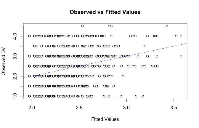
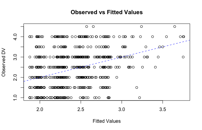
fitted_vals <- fitted(mod1)

# Plot observed values against fitted values
plot(fitted_vals, scale_scores$criticism_items_G_mean,
     xlab = "Fitted Values",
     ylab = "Observed DV",
     main = "Observed vs Fitted Values")
abline(0, 1, col = "blue", lty = 2)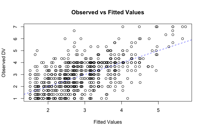

paste0("####################################################")

## [1] "####################################################"

paste0("REPORTS for each model (please ignore the eta squares, they are way off")

## [1] "REPORTS for each model (please ignore the eta squares, they are way off"

paste0("####################################################")

## [1] "####################################################"

paste0("MODEL 1: criticism_items_G_mean ~ Heroism")

## [1] "MODEL 1: criticism_items_G_mean ~ Heroism"

report(Anova(mod1 <- lm(criticism_items_G_mean ~ Heroism  + Cond, data = scale_scores), type = "III"))

## The ANOVA suggests that:
## 
##   - The main effect of Heroism is statistically significant and large (F(1, 833)
## = 354.95, p < .001; Eta2 (partial) = 0.30, 95% CI [0.26, 1.00])
##   - The main effect of Cond is statistically not significant and very small (F(5,
## 833) = 1.28, p = 0.271; Eta2 (partial) = 7.62e-03, 95% CI [0.00, 1.00])
## 
## Effect sizes were labelled following Field's (2013) recommendations.

paste0("MODEL 2: criticism_items_G_mean ~ Heroism * Cond")

## [1] "MODEL 2: criticism_items_G_mean ~ Heroism * Cond"

report(Anova(mod2 <- lm(criticism_items_G_mean ~ Heroism * Cond, data = scale_scores), type = "III"))

## Type 3 ANOVAs only give sensible and informative results when covariates
##   are mean-centered and factors are coded with orthogonal contrasts (such
##   as those produced by `contr.sum`, `contr.poly`, or `contr.helmert`, but
##   *not* by the default `contr.treatment`).

## The ANOVA suggests that:
## 
##   - The main effect of Heroism is statistically significant and large (F(1, 828)
## = 328.15, p < .001; Eta2 (partial) = 0.28, 95% CI [0.24, 1.00])
##   - The main effect of Cond is statistically not significant and very small (F(5,
## 828) = 0.97, p = 0.433; Eta2 (partial) = 5.84e-03, 95% CI [0.00, 1.00])
##   - The interaction between Heroism and Cond is statistically not significant and
## very small (F(5, 828) = 1.25, p = 0.286; Eta2 (partial) = 7.47e-03, 95% CI
## [0.00, 1.00])
## 
## Effect sizes were labelled following Field's (2013) recommendations.

paste0("MODEL 3: criticism_items_G_mean ~ Heroism +scale(Attitude)")

## [1] "MODEL 3: criticism_items_G_mean ~ Heroism +scale(Attitude)"

report(Anova(mod3 <- lm(criticism_items_G_mean ~ Heroism   + Cond +scale(Attitude) , data = scale_scores), type = "III"))

## The ANOVA suggests that:
## 
##   - The main effect of Heroism is statistically significant and small (F(1, 832)
## = 44.46, p < .001; Eta2 (partial) = 0.05, 95% CI [0.03, 1.00])
##   - The main effect of Cond is statistically not significant and very small (F(5,
## 832) = 1.48, p = 0.195; Eta2 (partial) = 8.80e-03, 95% CI [0.00, 1.00])
##   - The main effect of scale(Attitude) is statistically significant and medium
## (F(1, 832) = 115.16, p < .001; Eta2 (partial) = 0.12, 95% CI [0.09, 1.00])
## 
## Effect sizes were labelled following Field's (2013) recommendations.

paste0("MODEL 4: criticism_items_G_mean ~ Heroism * Cond + scale(Attitude)")

## [1] "MODEL 4: criticism_items_G_mean ~ Heroism * Cond + scale(Attitude)"

report(Anova(mod4 <-lm(criticism_items_G_mean ~ Heroism * Cond + scale(Attitude), data = scale_scores), type = "III"))

## Type 3 ANOVAs only give sensible and informative results when covariates
##   are mean-centered and factors are coded with orthogonal contrasts (such
##   as those produced by `contr.sum`, `contr.poly`, or `contr.helmert`, but
##   *not* by the default `contr.treatment`).

## The ANOVA suggests that:
## 
##   - The main effect of Heroism is statistically significant and small (F(1, 827)
## = 43.54, p < .001; Eta2 (partial) = 0.05, 95% CI [0.03, 1.00])
##   - The main effect of Cond is statistically not significant and very small (F(5,
## 827) = 1.30, p = 0.263; Eta2 (partial) = 7.78e-03, 95% CI [0.00, 1.00])
##   - The main effect of scale(Attitude) is statistically significant and medium
## (F(1, 827) = 114.47, p < .001; Eta2 (partial) = 0.12, 95% CI [0.09, 1.00])
##   - The interaction between Heroism and Cond is statistically not significant and
## very small (F(5, 827) = 1.24, p = 0.286; Eta2 (partial) = 7.47e-03, 95% CI
## [0.00, 1.00])
## 
## Effect sizes were labelled following Field's (2013) recommendations.

paste0("Model Comparison: assessing the importance of attitude - not accounting for occupations")

## [1] "Model Comparison: assessing the importance of attitude - not accounting for occupations"

anova(mod1, mod3)

paste0("Model Comparison: assessing the importance of attitude - accounting for occupations")

## [1] "Model Comparison: assessing the importance of attitude - accounting for occupations"

anova(mod2, mod4)

ggplot(scale_scores, aes(y = criticism_items_G_mean, x = Heroism)) +
  # 1) points colored by Cond
  geom_point(aes(color = Cond),
             size = 2.7, alpha = 0.7) +
  
  # 2) ONE global lm line (group = 1 prevents one line per Cond)
  stat_smooth(method = "lm", se = TRUE,
              aes(group = 1),
              color = "black", linewidth = 1) +
  
  # Nice, accessible palette (works well with >3 groups)
  scale_color_brewer(palette = "Set2") +
  
  labs(
    y = "Criticism accept. (G)",
    x = "Heroism",
    color = "Occupation",
    title = "Heroism vs. Criticism accept. (G), colored by Occupation",
    subtitle = "Points are participants; black line is overall linear fit with 95% CI"
  ) +
  theme_minimal(base_size = 12) +
  theme(
    legend.position = "right",
    panel.grid.minor = element_blank()
  )

## `geom_smooth()` using formula = 'y ~ x'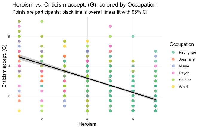

ggplot(scale_scores, aes(y = criticism_items_G_mean, x = Heroism, color = Cond)) +
  # points colored by condition
  geom_point(size = 2.7, alpha = 0.7) +
  # ONE lm line PER condition (because color is mapped here)
  stat_smooth(method = "lm", se = FALSE, linewidth = 1, fullrange = TRUE) +
  scale_color_brewer(palette = "Set2") +
  labs(
    y = "Criticism accept. (G)",
    x = "Heroism",
    color = "Occupation",
    title = "Heroism vs. Criticism accept. (G) with per-Occupation linear fits"
  ) +
  theme_minimal(base_size = 12) +
  theme(legend.position = "right", panel.grid.minor = element_blank())

## `geom_smooth()` using formula = 'y ~ x'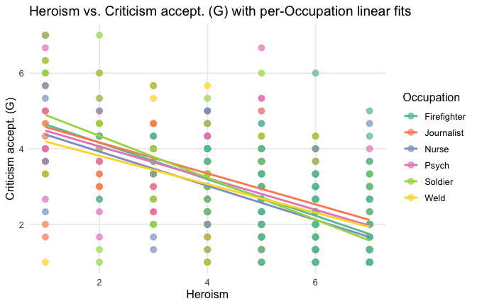

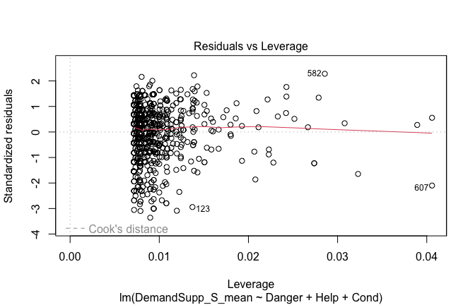
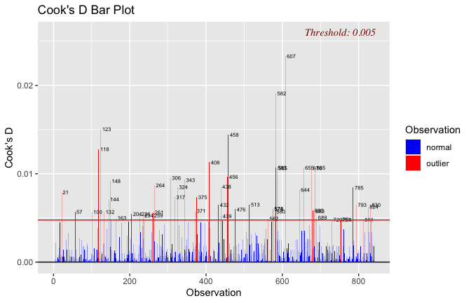
pal6 <- c("#800020", "#4E5BA6", "#1B7F79", "#4F718E", "#7A8F3E", "#B38E22")
pal6_alpha <- ggplot2::alpha(pal6, 0.7)   # <- bake in transparency

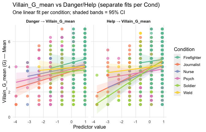
ggplot(scale_scores, aes(x = Heroism, y = Gratitude_G_mean)) +
  # 1) PER-CONDITION lines FIRST (go behind; already semi-transparent)
  stat_smooth(
    aes(color = Cond),
    method = "lm", se = FALSE, fullrange = TRUE,
    linewidth = 0.9, lineend = "round"
  ) +
  # 2) OVERALL black line + grey CI on top
  stat_smooth(
    method = "lm", se = TRUE, fullrange = TRUE,
    color = "black", fill = "grey30",
    alpha = 0.22, linewidth = 1.6
  ) +
  scale_color_manual(values = pal6_alpha, name = "Occupation") +
  # keep legend lines opaque for readability there
  guides(color = guide_legend(override.aes = list(alpha = 1, linewidth = 1.2))) +
  labs(
    x = "Heroism", y = "Gratitude",
  ) +
 geom_point(size = 2, alpha = 0.25, color = "black", show.legend = FALSE) +
  theme_minimal(base_size = 18) +
  theme(
    panel.grid.minor = element_blank(),
    panel.grid.major.x = element_blank(),
    plot.title = element_text(face = "bold")
  )

## `geom_smooth()` using formula = 'y ~ x'
## `geom_smooth()` using formula = 'y ~ x'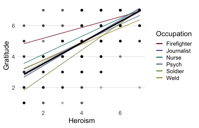

Overall: Heroism predict decreased general acceptability of criticism. This is true above and beyond attitude (see Model 3). It is true when controlling for normative effects of occupations (Model 2), and when controlling for both occupations and attitude (Model 4). See Summary table:

Model 1: “~Heroism + Occupation”

# =========================
# OLD MODELS (Heroism)
# =========================
m1_H <- lm(criticism_items_G_mean ~ Heroism + Occupation, data = scale_scores)
m2_H <- lm(criticism_items_G_mean ~ Heroism * Occupation, data = scale_scores)
m3_H <- lm(criticism_items_G_mean ~ Heroism + Occupation + Attitude, data = scale_scores)
m4_H <- lm(criticism_items_G_mean ~ Heroism * Occupation + Attitude, data = scale_scores)

tidy_type3(m1_H, "~Heroism + Cond")

~Heroism + Cond
	Term	df1	df2	F	p	eta2p
Heroism	Heroism	1	833	354.95	< .001	0.299
Occupation	Occupation	5	833	1.28	= 0.271	0.008

# =========================
# NEW MODELS (Danger & Help)
# =========================

Model 2: “~Heroism * Occupation”

tidy_type3(m2_H, "~Heroism * Cond")

~Heroism * Cond
	Term	df1	df2	F	p	eta2p
Heroism	Heroism	1	828	328.15	< .001	0.284
Occupation	Occupation	5	828	0.97	= 0.433	0.006
Heroism:Occupation	Heroism:Occupation	5	828	1.25	= 0.286	0.007

Model 3: “~Heroism + Occupation + Attitude”

tidy_type3(m3_H, "~Heroism + Occupation + Attitude")

~Heroism + Occupation + Attitude
	Term	df1	df2	F	p	eta2p
Heroism	Heroism	1	832	44.46	< .001	0.051
Occupation	Occupation	5	832	1.48	= 0.195	0.009
Attitude	Attitude	1	832	115.16	< .001	0.122

Model 4: “~Heroism * Occupation + Attitude”

tidy_type3(m4_H, "~Heroism * Occupation + Attitude")

~Heroism * Occupation + Attitude
	Term	df1	df2	F	p	eta2p
Heroism	Heroism	1	827	43.54	< .001	0.050
Occupation	Occupation	5	827	1.30	= 0.263	0.008
Attitude	Attitude	1	827	114.47	< .001	0.122
Heroism:Occupation	Heroism:Occupation	5	827	1.24	= 0.286	0.007

Comparison of main predictors across models

# Use orthogonal contrasts; keeps your "Heroism main effect" interpretable with Cond in the model
old_contr <- options(contrasts = c("contr.sum", "contr.poly"))

# Helper to extract the main effect of "Heroism" from a car::Anova table
extract_heroism <- function(mod, model_label) {
  a <- car::Anova(mod, type = "III")

  # Coerce to data.frame with rownames preserved
  tab <- as.data.frame(a)
  tab$Term <- rownames(tab)

  # Standard column names across R versions
  # (car::Anova uses these names for lm/glm type=III)
  # Columns: "Sum Sq", "Df", "F value", "Pr(>F)"
  names(tab) <- sub(" ", "_", names(tab))  # make names safe: "Sum_Sq", "F_value", etc.

  # Pull rows we need
  hero <- tab %>% filter(Term == "Heroism")
  resid <- tab %>% filter(Term == "Residuals")

  # Safety checks (in case of name variants)
  stopifnot(nrow(hero) == 1, nrow(resid) == 1)

  # Partial eta^2 = SS_effect / (SS_effect + SS_residual)
  eta_p2 <- hero$Sum_Sq / (hero$Sum_Sq + resid$Sum_Sq)

  # Format p nicely (APA-ish)
  p_fmt <- ifelse(hero$`Pr(>F)` < .001, "< .001",
                  sprintf("= %.3f", hero$`Pr(>F)`))

  dplyr::tibble(
    Model = model_label,
    Outcome = "criticism_items_G_mean",
    Predictor = "Heroism",
    df1 = hero$Df,
    df2 = resid$Df,
    F = hero$F_value,
    p = p_fmt,
    eta2p = eta_p2
  )
}

# ----- Fit the four models -----
mod1 <- lm(criticism_items_G_mean ~ Heroism   + Cond, data = scale_scores)
mod2 <- lm(criticism_items_G_mean ~ Heroism * Cond, data = scale_scores)
mod3 <- lm(criticism_items_G_mean ~ Heroism   + Cond + scale(Attitude), data = scale_scores)
mod4 <- lm(criticism_items_G_mean ~ Heroism * Cond + scale(Attitude), data = scale_scores)

# ----- Build the summary table -----
tbl <- bind_rows(
  extract_heroism(mod1, "~ Heroism   + Cond"),
  extract_heroism(mod2, "~ Heroism * Occupation"),
  extract_heroism(mod3, "~ Heroism   + Cond + Attitude"),
  extract_heroism(mod4, "~ Heroism * Occupation + Attitude")
  ) %>%
  # Nice number formatting for F and eta^2p
  mutate(
    F = round(F, 2),
    eta2p = round(eta2p, 3)
  )

# ----- Print as HTML-friendly table -----
# Build the table first
tbl_kbl <- tbl %>%
  kable("html",
        caption = "Main effect of Heroism across models (Type-III ANOVA): F, p, partial η²",
        align = "lllrrrcr")
# Add a footnote in a version-robust way
if ("footnote" %in% getNamespaceExports("kableExtra")) {
  tbl_kbl <- tbl_kbl %>%
    kableExtra::footnote(
      general = "Type-III sums of squares with sum contrasts. Partial η² = SS_effect / (SS_effect + SS_residual). p values are APA-style.",
      general_title = ""
    )
} else {
  tbl_kbl <- tbl_kbl %>%
    kableExtra::add_footnote(
      label = "Type-III sums of squares with sum contrasts. Partial η² = SS_effect / (SS_effect + SS_residual). p values are APA-style.",
      notation = "none"
    )
}

tbl_kbl

Main effect of Heroism across models (Type-III ANOVA): F, p, partial η²
Model	Outcome	Predictor	df1	df2	F	p	eta2p
~ Heroism + Cond	criticism_items_G_mean	Heroism	1	833	354.95	< .001	0.299
~ Heroism * Occupation	criticism_items_G_mean	Heroism	1	828	328.15	< .001	0.284
~ Heroism + Cond + Attitude	criticism_items_G_mean	Heroism	1	832	44.46	< .001	0.051
~ Heroism * Occupation + Attitude	criticism_items_G_mean	Heroism	1	827	43.54	< .001	0.050
Type-III sums of squares with sum contrasts. Partial η² = SS_effect / (SS_effect + SS_residual). p values are APA-style.

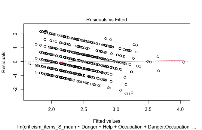
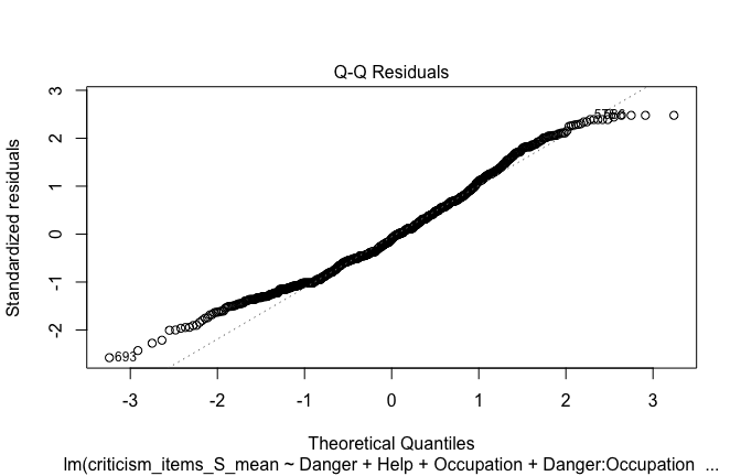
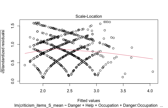
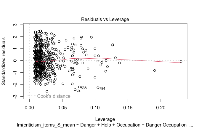
Specific level

[An online post that says: “Journalists are evil and wish harm on other people”] The person making this post should be prosecuted using the UK laws against “grossly offensive” public messaging

Toggle details of the models diagnostics and outlier analyses

Below, you’ll find model diagnostics (QQ plot, fitted vs residuals, linearity), Outliers analysis, and more details on the output

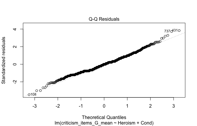
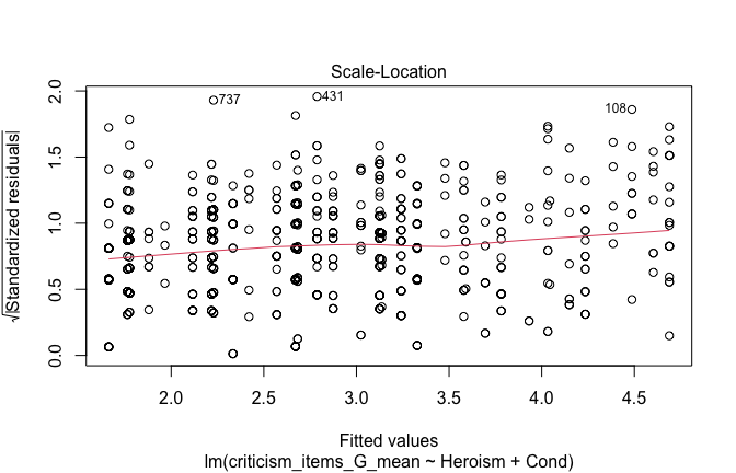
[NOTE THAT EFFECT SIZES REPORTED IN THE REPORT COMMANDS BELOW SHOULD NOT BE TRUSTED]

paste0("####################################################")

## [1] "####################################################"

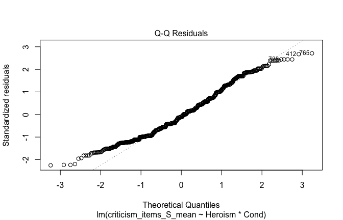
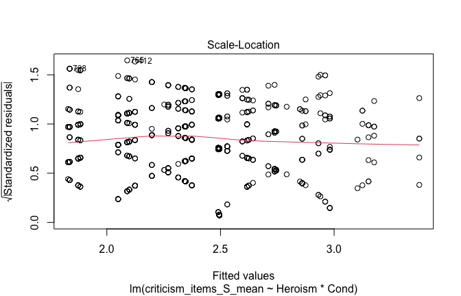
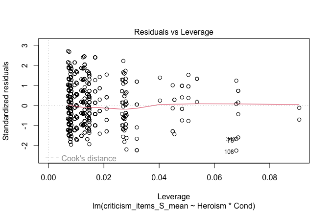
paste0("Diagnostics for Model 1: DV ~ Heroism + Occupation")

## [1] "Diagnostics for Model 1: DV ~ Heroism + Occupation"

paste0("####################################################")

## [1] "####################################################"

mod1 <- lm(criticism_items_S_mean ~ Heroism  + Cond, data = scale_scores, na.action = na.exclude)
mod1r <- lmrob(criticism_items_S_mean ~ Heroism  + Cond, data = scale_scores, na.action = na.exclude)
plot(mod1)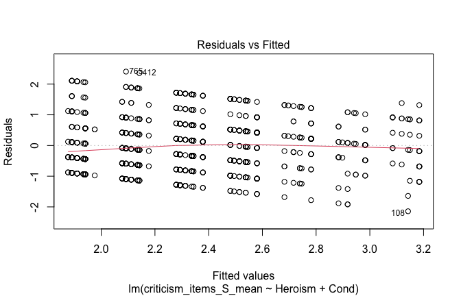

ols_plot_cooksd_bar(mod1, type = 1)

paste0("Comparison with Robust model")

## [1] "Comparison with Robust model"

models <- list("OLS (lm)" = mod1, "Robust (lmrob)" = mod1r)
modelsummary(
  models,
  statistic = c("({std.error})", "{statistic}", "p = {p.value}"),
  gof_omit  = "IC|Log.Lik",   # robust AIC comparability is iffy; omit by default
  output    = "html"
)

## Warning in w * res^2: longer object length is not a multiple of shorter object
## length

## Warning in log(w) - (log(2 * pi) + log(s2) + (w * res^2)/s2): longer object
## length is not a multiple of shorter object length

	OLS (lm)	Robust (lmrob)
(Intercept)	3.331	3.397
	(0.109)	(0.117)
	30.608	28.949
	p = <0.001	p = <0.001
Heroism	−0.201	−0.223
	(0.021)	(0.023)
	−9.496	−9.776
	p = <0.001	p = <0.001
Cond1	−0.031	−0.047
	(0.072)	(0.082)
	−0.425	−0.573
	p = 0.671	p = 0.567
Cond2	0.054	0.070
	(0.075)	(0.073)
	0.725	0.951
	p = 0.469	p = 0.342
Cond3	0.019	0.041
	(0.070)	(0.068)
	0.275	0.598
	p = 0.784	p = 0.550
Cond4	−0.045	−0.037
	(0.069)	(0.075)
	−0.645	−0.497
	p = 0.519	p = 0.619
Cond5	−0.011	−0.022
	(0.069)	(0.080)
	−0.158	−0.280
	p = 0.874	p = 0.780
Num.Obs.	838	838
R2	0.129	0.151
R2 Adj.	0.123	0.145
RMSE	0.89	0.89

fitted_vals <- fitted(mod1)

# Plot observed values against fitted values
plot(fitted_vals, scale_scores$criticism_items_S_mean,
     xlab = "Fitted Values",
     ylab = "Observed DV",
     main = "Observed vs Fitted Values")
abline(0, 1, col = "blue", lty = 2)

paste0("####################################################")

## [1] "####################################################"

paste0("Diagnostics for Model 2: DV ~ Heroism * Occupation")

## [1] "Diagnostics for Model 2: DV ~ Heroism * Occupation"

paste0("####################################################")

## [1] "####################################################"

mod1 <- lm(criticism_items_S_mean ~ Heroism  * Cond, data = scale_scores, na.action = na.exclude)
mod1r <- lmrob(criticism_items_S_mean ~ Heroism  * Cond, data = scale_scores, na.action = na.exclude)
plot(mod1)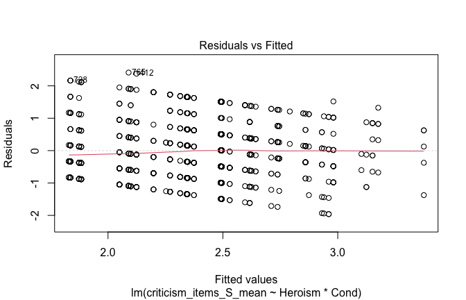

ols_plot_cooksd_bar(mod1, type = 1)

paste0("Comparison with Robust model")

## [1] "Comparison with Robust model"

models <- list("OLS (lm)" = mod1, "Robust (lmrob)" = mod1r)
modelsummary(
  models,
  statistic = c("({std.error})", "{statistic}", "p = {p.value}"),
  gof_omit  = "IC|Log.Lik",   # robust AIC comparability is iffy; omit by default
  output    = "html"
)

## Warning in w * res^2: longer object length is not a multiple of shorter object
## length
## Warning in w * res^2: longer object length is not a multiple of shorter object
## length

	OLS (lm)	Robust (lmrob)
(Intercept)	3.365	3.450
	(0.115)	(0.130)
	29.315	26.547
	p = <0.001	p = <0.001
Heroism	−0.202	−0.226
	(0.022)	(0.024)
	−9.232	−9.318
	p = <0.001	p = <0.001
Cond1	0.245	0.236
	(0.343)	(0.406)
	0.714	0.582
	p = 0.475	p = 0.561
Cond2	−0.262	−0.365
	(0.196)	(0.186)
	−1.340	−1.963
	p = 0.181	p = 0.050
Cond3	0.260	0.203
	(0.255)	(0.263)
	1.019	0.770
	p = 0.309	p = 0.441
Cond4	0.007	−0.026
	(0.230)	(0.222)
	0.030	−0.117
	p = 0.976	p = 0.907
Cond5	0.027	0.143
	(0.230)	(0.263)
	0.117	0.543
	p = 0.907	p = 0.587
Heroism × Cond1	−0.052	−0.054
	(0.058)	(0.066)
	−0.899	−0.820
	p = 0.369	p = 0.412
Heroism × Cond2	0.080	0.112
	(0.047)	(0.043)
	1.717	2.565
	p = 0.086	p = 0.010
Heroism × Cond3	−0.049	−0.035
	(0.045)	(0.045)
	−1.088	−0.791
	p = 0.277	p = 0.429
Heroism × Cond4	−0.019	−0.012
	(0.047)	(0.044)
	−0.397	−0.266
	p = 0.692	p = 0.790
Heroism × Cond5	−0.014	−0.041
	(0.043)	(0.049)
	−0.324	−0.838
	p = 0.746	p = 0.402
Num.Obs.	838	838
R2	0.134	0.162
R2 Adj.	0.123	0.151
RMSE	0.89	0.89

fitted_vals <- fitted(mod1)

# Plot observed values against fitted values
plot(fitted_vals, scale_scores$criticism_items_S_mean,
     xlab = "Fitted Values",
     ylab = "Observed DV",
     main = "Observed vs Fitted Values")
abline(0, 1, col = "blue", lty = 2)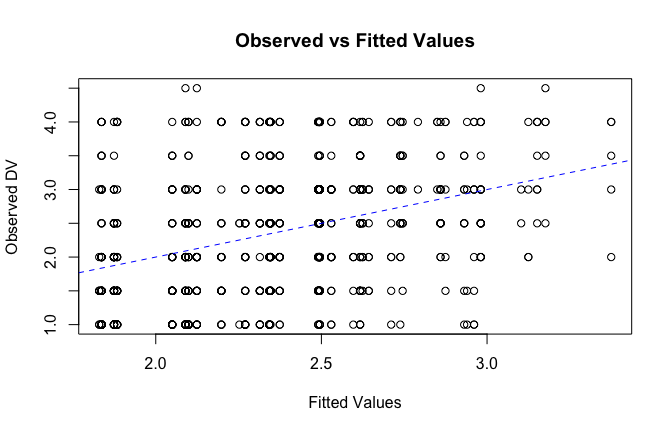

paste0("####################################################")

## [1] "####################################################"

paste0("Diagnostics for Model 3: DV ~ Heroism + Occupation + Attitude")

## [1] "Diagnostics for Model 3: DV ~ Heroism + Occupation + Attitude"

paste0("####################################################")

## [1] "####################################################"

mod1 <- lm(criticism_items_S_mean ~ Heroism  + Cond + Attitude, data = scale_scores, na.action = na.exclude)
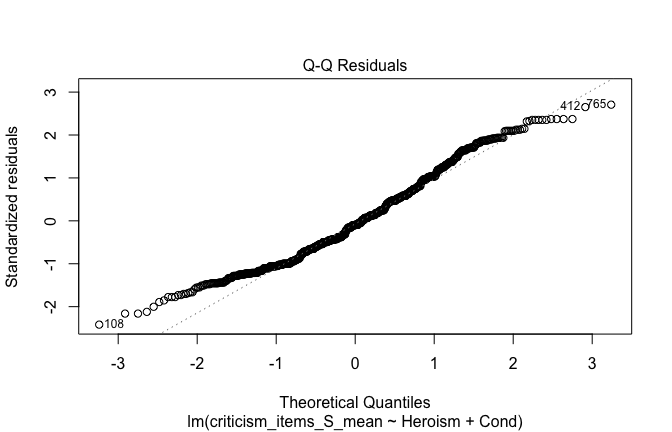
mod1r <- lmrob(criticism_items_S_mean ~ Heroism  + Cond + Attitude, data = scale_scores, na.action = na.exclude)
plot(mod1)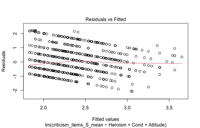

ols_plot_cooksd_bar(mod1, type = 1)

paste0("Comparison with Robust model")

## [1] "Comparison with Robust model"

models <- list("OLS (lm)" = mod1, "Robust (lmrob)" = mod1r)
modelsummary(
  models,
  statistic = c("({std.error})", "{statistic}", "p = {p.value}"),
  gof_omit  = "IC|Log.Lik",   # robust AIC comparability is iffy; omit by default
  output    = "html"
)

## Warning in w * res^2: longer object length is not a multiple of shorter object
## length
## Warning in w * res^2: longer object length is not a multiple of shorter object
## length

	OLS (lm)	Robust (lmrob)
(Intercept)	2.849	2.850
	(0.149)	(0.178)
	19.175	15.994
	p = <0.001	p = <0.001
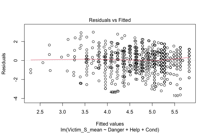
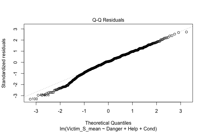
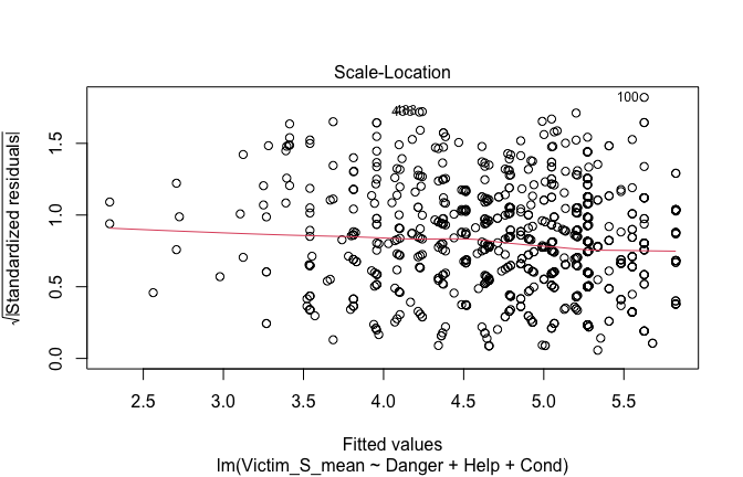
Heroism	−0.104	−0.112
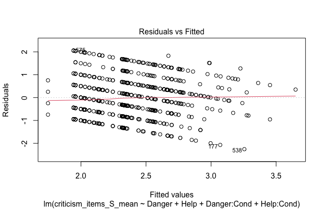
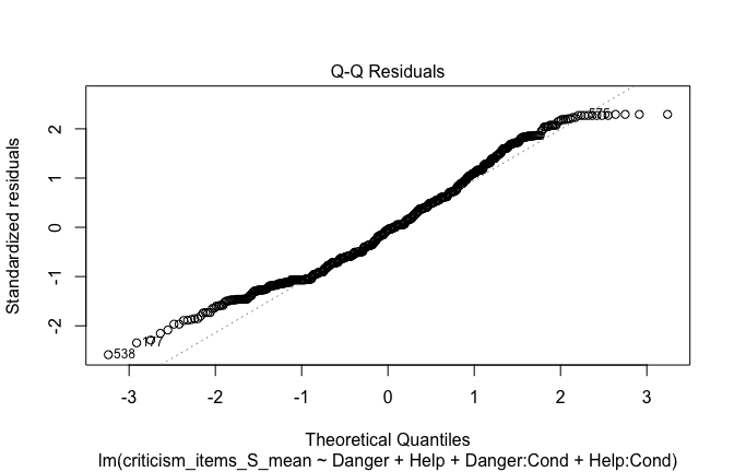
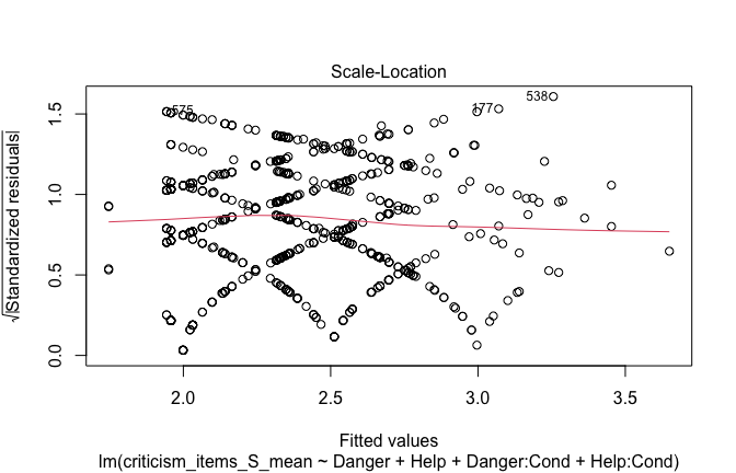
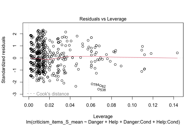
	(0.030)	(0.035)
	−3.508	−3.167
	p = <0.001	p = 0.002
Cond1	0.019	0.004
	(0.072)	(0.081)
	0.267	0.045
	p = 0.789	p = 0.964
Cond2	−0.023	−0.015
	(0.076)	(0.074)
	−0.306	−0.208
	p = 0.759	p = 0.835
Cond3	0.063	0.086
	(0.070)	(0.068)
	0.892	1.272
	p = 0.372	p = 0.204
Cond4	−0.020	−0.002
	(0.069)	(0.075)
	−0.295	−0.029
	p = 0.768	p = 0.977
Cond5	−0.051	−0.070
	(0.069)	(0.078)
	−0.745	−0.895
	p = 0.456	p = 0.371
Attitude	−0.233	−0.256
	(0.050)	(0.057)
	−4.705	−4.467
	p = <0.001	p = <0.001
Num.Obs.	838	838
R2	0.152	0.176
R2 Adj.	0.144	0.169
RMSE	0.88	0.88

fitted_vals <- fitted(mod1)

# Plot observed values against fitted values
plot(fitted_vals, scale_scores$criticism_items_S_mean,
     xlab = "Fitted Values",
     ylab = "Observed DV",
     main = "Observed vs Fitted Values")
abline(0, 1, col = "blue", lty = 2)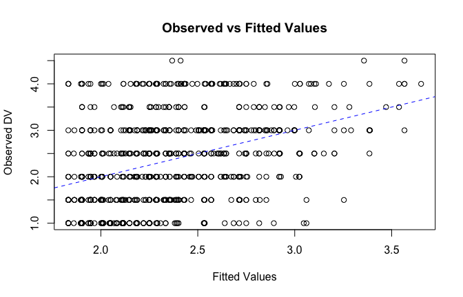

paste0("####################################################")

## [1] "####################################################"

paste0("Diagnostics for Model 4: DV ~ Heroism * Occupation + Attitude")

## [1] "Diagnostics for Model 4: DV ~ Heroism * Occupation + Attitude"

paste0("####################################################")

## [1] "####################################################"

mod1 <- lm(criticism_items_S_mean ~ Heroism*Cond + Attitude, data = scale_scores, na.action = na.exclude)
mod1r <- lmrob(criticism_items_S_mean ~ Heroism*Cond + Attitude, data = scale_scores, na.action = na.exclude)
plot(mod1)

ols_plot_cooksd_bar(mod1, type = 1)

paste0("Comparison with Robust model")

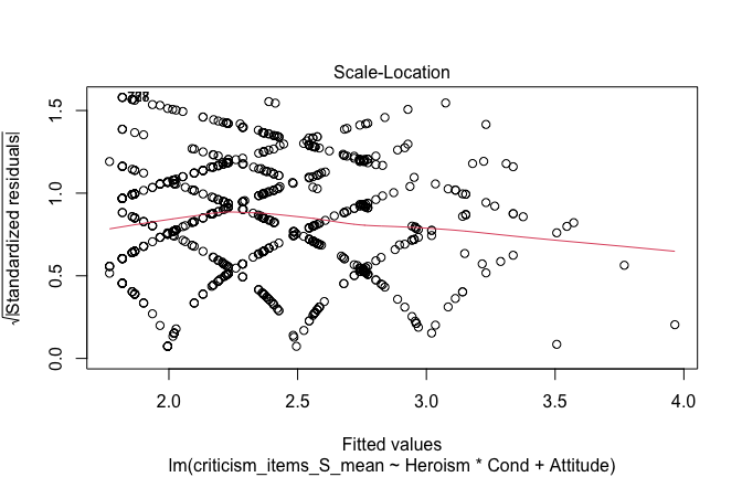
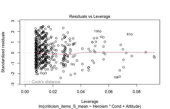
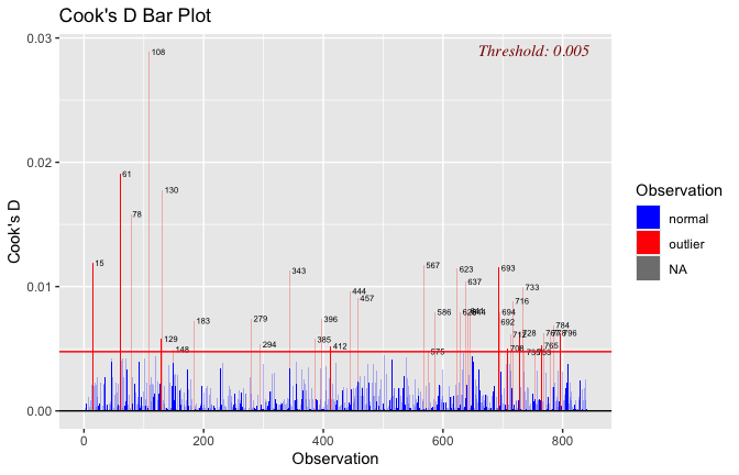
## [1] "Comparison with Robust model"

models <- list("OLS (lm)" = mod1, "Robust (lmrob)" = mod1r)
modelsummary(
  models,
  statistic = c("({std.error})", "{statistic}", "p = {p.value}"),
  gof_omit  = "IC|Log.Lik",   # robust AIC comparability is iffy; omit by default
  output    = "html"
)

## Warning in w * res^2: longer object length is not a multiple of shorter object
## length
## Warning in w * res^2: longer object length is not a multiple of shorter object
## length

	OLS (lm)	Robust (lmrob)
(Intercept)	2.868	2.892
	(0.150)	(0.184)
	19.064	15.746
	p = <0.001	p = <0.001
Heroism	−0.099	−0.111
	(0.030)	(0.036)
	−3.333	−3.088
	p = <0.001	p = 0.002
Cond1	0.444	0.459
	(0.340)	(0.394)
	1.303	1.166
	p = 0.193	p = 0.244
Cond2	−0.457	−0.549
	(0.197)	(0.169)
	−2.323	−3.249
	p = 0.020	p = 0.001
Cond3	0.332	0.261
	(0.252)	(0.255)
	1.318	1.022
	p = 0.188	p = 0.307
Cond4	0.088	0.056
	(0.228)	(0.224)
	0.389	0.251
	p = 0.698	p = 0.802
Cond5	−0.201	−0.105
	(0.231)	(0.240)
	−0.872	−0.437
	p = 0.383	p = 0.662
Attitude	−0.254	−0.276
	(0.051)	(0.058)
	−5.006	−4.766
	p = <0.001	p = <0.001
Heroism × Cond1	−0.077	−0.083
	(0.057)	(0.064)
	−1.350	−1.294
	p = 0.177	p = 0.196
Heroism × Cond2	0.107	0.135
	(0.046)	(0.039)
	2.316	3.412
	p = 0.021	p = <0.001
Heroism × Cond3	−0.054	−0.038
	(0.044)	(0.043)
	−1.230	−0.875
	p = 0.219	p = 0.382
Heroism × Cond4	−0.033	−0.024
	(0.047)	(0.045)
	−0.712	−0.535
	p = 0.477	p = 0.593
Heroism × Cond5	0.021	−0.004
	(0.043)	(0.045)
	0.479	−0.084
	p = 0.632	p = 0.933
Num.Obs.	838	838
R2	0.160	0.190
R2 Adj.	0.148	0.178
RMSE	0.87	0.88

fitted_vals <- fitted(mod1)

# Plot observed values against fitted values
plot(fitted_vals, scale_scores$criticism_items_S_mean,
     xlab = "Fitted Values",
     ylab = "Observed DV",
     main = "Observed vs Fitted Values")
abline(0, 1, col = "blue", lty = 2)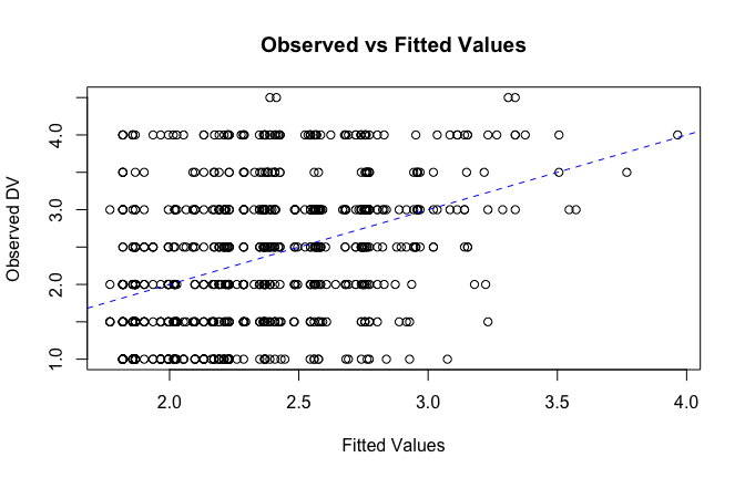

paste0("####################################################")

## [1] "####################################################"

paste0("REPORTS for each model (please ignore the eta squares, they are way off")

## [1] "REPORTS for each model (please ignore the eta squares, they are way off"

paste0("####################################################")

## [1] "####################################################"

paste0("MODEL 1: criticism_items_S_mean ~ Heroism")

## [1] "MODEL 1: criticism_items_S_mean ~ Heroism"

report(Anova(mod1 <- lm(criticism_items_S_mean ~ Heroism  + Cond, data = scale_scores), type = "III"))

## The ANOVA suggests that:
## 
##   - The main effect of Heroism is statistically significant and medium (F(1, 831)
## = 90.18, p < .001; Eta2 (partial) = 0.10, 95% CI [0.07, 1.00])
##   - The main effect of Cond is statistically not significant and very small (F(5,
## 831) = 0.22, p = 0.955; Eta2 (partial) = 1.30e-03, 95% CI [0.00, 1.00])
## 
## Effect sizes were labelled following Field's (2013) recommendations.

paste0("MODEL 2: criticism_items_S_mean ~ Heroism * Cond")

## [1] "MODEL 2: criticism_items_S_mean ~ Heroism * Cond"

report(Anova(mod2 <- lm(criticism_items_S_mean ~ Heroism * Cond, data = scale_scores), type = "III"))

## Type 3 ANOVAs only give sensible and informative results when covariates
##   are mean-centered and factors are coded with orthogonal contrasts (such
##   as those produced by `contr.sum`, `contr.poly`, or `contr.helmert`, but
##   *not* by the default `contr.treatment`).

## The ANOVA suggests that:
## 
##   - The main effect of Heroism is statistically significant and medium (F(1, 826)
## = 85.23, p < .001; Eta2 (partial) = 0.09, 95% CI [0.06, 1.00])
##   - The main effect of Cond is statistically not significant and very small (F(5,
## 826) = 0.75, p = 0.585; Eta2 (partial) = 4.53e-03, 95% CI [0.00, 1.00])
##   - The interaction between Heroism and Cond is statistically not significant and
## very small (F(5, 826) = 1.05, p = 0.386; Eta2 (partial) = 6.33e-03, 95% CI
## [0.00, 1.00])
## 
## Effect sizes were labelled following Field's (2013) recommendations.

paste0("MODEL 3: criticism_items_S_mean ~ Heroism +scale(Attitude)")

## [1] "MODEL 3: criticism_items_S_mean ~ Heroism +scale(Attitude)"

report(Anova(mod3 <- lm(criticism_items_S_mean ~ Heroism   + Cond +scale(Attitude) , data = scale_scores), type = "III"))

## The ANOVA suggests that:
## 
##   - The main effect of Heroism is statistically significant and small (F(1, 830)
## = 12.31, p < .001; Eta2 (partial) = 0.01, 95% CI [4.13e-03, 1.00])
##   - The main effect of Cond is statistically not significant and very small (F(5,
## 830) = 0.26, p = 0.935; Eta2 (partial) = 1.56e-03, 95% CI [0.00, 1.00])
##   - The main effect of scale(Attitude) is statistically significant and small
## (F(1, 830) = 22.14, p < .001; Eta2 (partial) = 0.03, 95% CI [0.01, 1.00])
## 
## Effect sizes were labelled following Field's (2013) recommendations.

paste0("MODEL 4: criticism_items_S_mean ~ Heroism * Cond + scale(Attitude)")

## [1] "MODEL 4: criticism_items_S_mean ~ Heroism * Cond + scale(Attitude)"

report(Anova(mod4 <-lm(criticism_items_S_mean ~ Heroism * Cond + scale(Attitude), data = scale_scores), type = "III"))

## Type 3 ANOVAs only give sensible and informative results when covariates
##   are mean-centered and factors are coded with orthogonal contrasts (such
##   as those produced by `contr.sum`, `contr.poly`, or `contr.helmert`, but
##   *not* by the default `contr.treatment`).

## The ANOVA suggests that:
## 
##   - The main effect of Heroism is statistically significant and small (F(1, 825)
## = 11.11, p < .001; Eta2 (partial) = 0.01, 95% CI [3.42e-03, 1.00])
##   - The main effect of Cond is statistically not significant and small (F(5, 825)
## = 1.67, p = 0.139; Eta2 (partial) = 0.01, 95% CI [0.00, 1.00])
##   - The main effect of scale(Attitude) is statistically significant and small
## (F(1, 825) = 25.06, p < .001; Eta2 (partial) = 0.03, 95% CI [0.01, 1.00])
##   - The interaction between Heroism and Cond is statistically not significant and
## very small (F(5, 825) = 1.65, p = 0.144; Eta2 (partial) = 9.90e-03, 95% CI
## [0.00, 1.00])
## 
## Effect sizes were labelled following Field's (2013) recommendations.

paste0("Model Comparison: assessing the importance of attitude - not accounting for occupations")

## [1] "Model Comparison: assessing the importance of attitude - not accounting for occupations"

anova(mod1, mod3)

paste0("Model Comparison: assessing the importance of attitude - accounting for occupations")

## [1] "Model Comparison: assessing the importance of attitude - accounting for occupations"

anova(mod2, mod4)

ggplot(scale_scores, aes(y = criticism_items_S_mean, x = Heroism)) +
  # 1) points colored by Cond
  geom_point(aes(color = Cond),
             size = 2.7, alpha = 0.7) +
  
  # 2) ONE global lm line (group = 1 prevents one line per Cond)
  stat_smooth(method = "lm", se = TRUE,
              aes(group = 1),
              color = "black", linewidth = 1) +
  
  # Nice, accessible palette (works well with >3 groups)
  scale_color_brewer(palette = "Set2") +
  
  labs(
    y = "Criticism accept. (S)",
    x = "Heroism",
    color = "Occupation",
    title = "Heroism vs. Criticism accept. (S), colored by Occupation",
    subtitle = "Points are participants; black line is overall linear fit with 95% CI"
  ) +
  theme_minimal(base_size = 12) +
  theme(
    legend.position = "right",
    panel.grid.minor = element_blank()
  )

## `geom_smooth()` using formula = 'y ~ x'

## Warning: Removed 2 rows containing non-finite outside the scale range
## (`stat_smooth()`).

## Warning: Removed 2 rows containing missing values or values outside the scale range
## (`geom_point()`).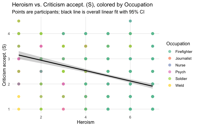

ggplot(scale_scores, aes(y = criticism_items_S_mean, x = Heroism, color = Cond)) +
  # points colored by condition
  geom_point(size = 2.7, alpha = 0.7) +
  # ONE lm line PER condition (because color is mapped here)
  stat_smooth(method = "lm", se = FALSE, linewidth = 1, fullrange = TRUE) +
  scale_color_brewer(palette = "Set2") +
  labs(
    y = "Criticism accept. (S)",
    x = "Heroism",
    color = "Occupation",
    title = "Heroism vs. Criticism accept. (S) with per-Occupation linear fits"
  ) +
  theme_minimal(base_size = 12) +
  theme(legend.position = "right", panel.grid.minor = element_blank())

## `geom_smooth()` using formula = 'y ~ x'

## Warning: Removed 2 rows containing non-finite outside the scale range (`stat_smooth()`).
## Removed 2 rows containing missing values or values outside the scale range
## (`geom_point()`).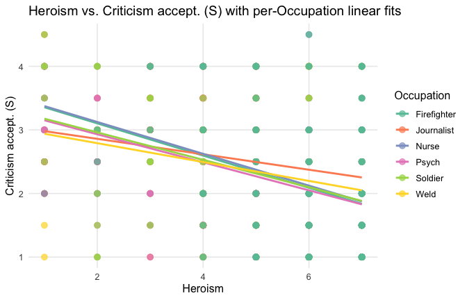

Overall: Heroism predict decreased specific acceptability of criticism. This is true above and beyond attitude (see Model 3)– Although effect sizes are drastically reduced when accounting for attitude in the case of specific acceptability of criticism. It is true when controlling for normative effects of occupations (Model 2), and when controlling for both occupations and attitude (Model 4). See Summary table:

Model 1: “~Heroism + Occupation”

# =========================
# OLD MODELS (Heroism)
# =========================
m1_H <- lm(criticism_items_S_mean ~ Heroism + Occupation, data = scale_scores)
m2_H <- lm(criticism_items_S_mean ~ Heroism * Occupation, data = scale_scores)
m3_H <- lm(criticism_items_S_mean ~ Heroism + Occupation + Attitude, data = scale_scores)
m4_H <- lm(criticism_items_S_mean ~ Heroism * Occupation + Attitude, data = scale_scores)

tidy_type3(m1_H, "~Heroism + Cond")

~Heroism + Cond
	Term	df1	df2	F	p	eta2p
Heroism	Heroism	1	831	90.18	< .001	0.098
Occupation	Occupation	5	831	0.22	= 0.955	0.001

# =========================
# NEW MODELS (Danger & Help)
# =========================

Model 2: “~Heroism * Occupation”

tidy_type3(m2_H, "~Heroism * Cond")

~Heroism * Cond
	Term	df1	df2	F	p	eta2p
Heroism	Heroism	1	826	85.23	< .001	0.094
Occupation	Occupation	5	826	0.75	= 0.585	0.005
Heroism:Occupation	Heroism:Occupation	5	826	1.05	= 0.386	0.006

Model 3: “~Heroism + Occupation + Attitude”

tidy_type3(m3_H, "~Heroism + Occupation + Attitude")

~Heroism + Occupation + Attitude
	Term	df1	df2	F	p	eta2p
Heroism	Heroism	1	830	12.31	< .001	0.015
Occupation	Occupation	5	830	0.26	= 0.935	0.002
Attitude	Attitude	1	830	22.14	< .001	0.026

Model 4: “~Heroism * Occupation + Attitude”

tidy_type3(m4_H, "~Heroism * Occupation + Attitude")

~Heroism * Occupation + Attitude
	Term	df1	df2	F	p	eta2p
Heroism	Heroism	1	825	11.11	< .001	0.013
Occupation	Occupation	5	825	1.67	= 0.139	0.010
Attitude	Attitude	1	825	25.06	< .001	0.029
Heroism:Occupation	Heroism:Occupation	5	825	1.65	= 0.144	0.010

Comparison of main predictors across models

# Use orthogonal contrasts; keeps your "Heroism main effect" interpretable with Cond in the model
old_contr <- options(contrasts = c("contr.sum", "contr.poly"))

# Helper to extract the main effect of "Heroism" from a car::Anova table
extract_heroism <- function(mod, model_label) {
  a <- car::Anova(mod, type = "III")

  # Coerce to data.frame with rownames preserved
  tab <- as.data.frame(a)
  tab$Term <- rownames(tab)

  # Standard column names across R versions
  # (car::Anova uses these names for lm/glm type=III)
  # Columns: "Sum Sq", "Df", "F value", "Pr(>F)"
  names(tab) <- sub(" ", "_", names(tab))  # make names safe: "Sum_Sq", "F_value", etc.

  # Pull rows we need
  hero <- tab %>% filter(Term == "Heroism")
  resid <- tab %>% filter(Term == "Residuals")

  # Safety checks (in case of name variants)
  stopifnot(nrow(hero) == 1, nrow(resid) == 1)

  # Partial eta^2 = SS_effect / (SS_effect + SS_residual)
  eta_p2 <- hero$Sum_Sq / (hero$Sum_Sq + resid$Sum_Sq)

  # Format p nicely (APA-ish)
  p_fmt <- ifelse(hero$`Pr(>F)` < .001, "< .001",
                  sprintf("= %.3f", hero$`Pr(>F)`))

  dplyr::tibble(
    Model = model_label,
    Outcome = "criticism_items_S_mean",
    Predictor = "Heroism",
    df1 = hero$Df,
    df2 = resid$Df,
    F = hero$F_value,
    p = p_fmt,
    eta2p = eta_p2
  )
}

# ----- Fit the four models -----
mod1 <- lm(criticism_items_S_mean ~ Heroism   + Cond, data = scale_scores)
mod2 <- lm(criticism_items_S_mean ~ Heroism * Cond, data = scale_scores)
mod3 <- lm(criticism_items_S_mean ~ Heroism  + Cond+ scale(Attitude), data = scale_scores)
mod4 <- lm(criticism_items_S_mean ~ Heroism * Cond + scale(Attitude), data = scale_scores)

# ----- Build the summary table -----
tbl <- bind_rows(
  extract_heroism(mod1, "~ Heroism + Cond"),
  extract_heroism(mod2, "~ Heroism * Occupation"),
  extract_heroism(mod3, "~ Heroism + Cond + Attitude"),
  extract_heroism(mod4, "~ Heroism * Occupation + Attitude")
  ) %>%
  # Nice number formatting for F and eta^2p
  mutate(
    F = round(F, 2),
    eta2p = round(eta2p, 3)
  )

# ----- Print as HTML-friendly table -----
# Build the table first
tbl_kbl <- tbl %>%
  kable("html",
        caption = "Main effect of Heroism across models (Type-III ANOVA): F, p, partial η²",
        align = "lllrrrcr")
# Add a footnote in a version-robust way
if ("footnote" %in% getNamespaceExports("kableExtra")) {
  tbl_kbl <- tbl_kbl %>%
    kableExtra::footnote(
      general = "Type-III sums of squares with sum contrasts. Partial η² = SS_effect / (SS_effect + SS_residual). p values are APA-style.",
      general_title = ""
    )
} else {
  tbl_kbl <- tbl_kbl %>%
    kableExtra::add_footnote(
      label = "Type-III sums of squares with sum contrasts. Partial η² = SS_effect / (SS_effect + SS_residual). p values are APA-style.",
      notation = "none"
    )
}

tbl_kbl

Main effect of Heroism across models (Type-III ANOVA): F, p, partial η²
Model	Outcome	Predictor	df1	df2	F	p	eta2p
~ Heroism + Cond	criticism_items_S_mean	Heroism	1	831	90.18	< .001	0.098
~ Heroism * Occupation	criticism_items_S_mean	Heroism	1	826	85.23	< .001	0.094
~ Heroism + Cond + Attitude	criticism_items_S_mean	Heroism	1	830	12.31	< .001	0.015
~ Heroism * Occupation + Attitude	criticism_items_S_mean	Heroism	1	825	11.11	< .001	0.013
Type-III sums of squares with sum contrasts. Partial η² = SS_effect / (SS_effect + SS_residual). p values are APA-style.

==> Full support for our hypotheses. Across all occupations Heroism predict general- and specific-level acceptability of criticism, with or without controlling for attitude.

H3: Heroism is associated with reduced support for demands from workers

Because it is expected from heroes to be selfless, demands from workers are incompatible with the hero status and should be evaluated negatively. This is a backlash from the heroic status that parallels previous findings on the exploitation of heroes (see Stanley & Kay, 2024). At the general level, it means reporting that it is justified for workers to take the lead (vs the government to take the lead) on pushing demands to improve their situation. At the specific level, it means supporting the right for workers to protest and make demands to improve their working situation.

General level

[it is justified for] XXX, and not the government, to take the lead on improvements that benefit the profession

Toggle details of the models diagnostics and outlier analyses

Below, you’ll find model diagnostics (QQ plot, fitted vs residuals, linearity), Outliers analysis, and more details on the output

[NOTE THAT EFFECT SIZES REPORTED IN THE REPORT COMMANDS BELOW SHOULD NOT BE TRUSTED]

paste0("####################################################")

## [1] "####################################################"

paste0("Diagnostics for Model 1: DV ~ Heroism + Occupation")

## [1] "Diagnostics for Model 1: DV ~ Heroism + Occupation"

paste0("####################################################")

## [1] "####################################################"

mod1 <- lm(DemandSupp_G_mean ~ Heroism  + Cond, data = scale_scores)
mod1r <- lmrob(DemandSupp_G_mean ~ Heroism  + Cond, data = scale_scores)
plot(mod1)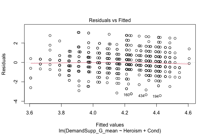

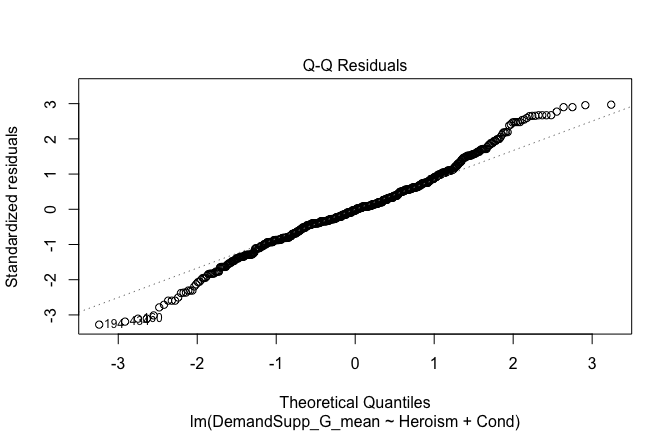
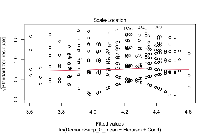
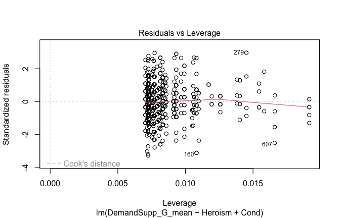
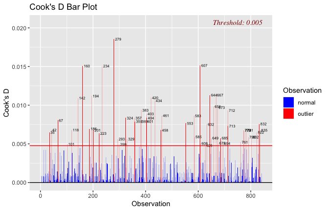
ols_plot_cooksd_bar(mod1, type = 1)

paste0("Comparison with Robust model")

## [1] "Comparison with Robust model"

models <- list("OLS (lm)" = mod1, "Robust (lmrob)" = mod1r)
modelsummary(
  models,
  statistic = c("({std.error})", "{statistic}", "p = {p.value}"),
  gof_omit  = "IC|Log.Lik",   # robust AIC comparability is iffy; omit by default
  output    = "html"
)

	OLS (lm)	Robust (lmrob)
(Intercept)	3.897	3.920
	(0.128)	(0.121)
	30.509	32.351
	p = <0.001	p = <0.001
Heroism	0.061	0.052
	(0.025)	(0.025)
	2.447	2.088
	p = 0.015	p = 0.037
Cond1	0.089	0.021
	(0.084)	(0.087)
	1.053	0.237
	p = 0.293	p = 0.813
Cond2	0.282	0.308
	(0.088)	(0.077)
	3.217	3.992
	p = 0.001	p = <0.001
Cond3	−0.113	−0.074
	(0.083)	(0.087)
	−1.363	−0.856
	p = 0.173	p = 0.392
Cond4	0.193	0.203
	(0.081)	(0.070)
	2.375	2.897
	p = 0.018	p = 0.004
Cond5	−0.352	−0.356
	(0.081)	(0.078)
	−4.315	−4.554
	p = <0.001	p = <0.001
Num.Obs.	840	840
R2	0.040	0.047
R2 Adj.	0.033	0.040
RMSE	1.04	1.05

fitted_vals <- fitted(mod1)

# Plot observed values against fitted values
plot(fitted_vals, scale_scores$DemandSupp_G_mean,
     xlab = "Fitted Values",
     ylab = "Observed DV",
     main = "Observed vs Fitted Values")
abline(0, 1, col = "blue", lty = 2)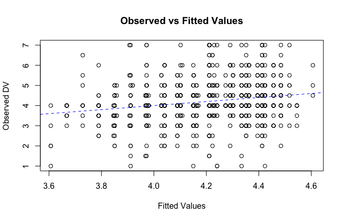

paste0("####################################################")

## [1] "####################################################"

paste0("Diagnostics for Model 2: DV ~ Heroism * Occupation")

## [1] "Diagnostics for Model 2: DV ~ Heroism * Occupation"

paste0("####################################################")

## [1] "####################################################"

mod1 <- lm(DemandSupp_G_mean ~ Heroism  * Cond, data = scale_scores)
mod1r <- lmrob(DemandSupp_G_mean ~ Heroism  * Cond, data = scale_scores)

## Warning in lmrob.S(x, y, control = control): S refinements did not converge (to
## refine.tol=1e-07) in 200 (= k.max) steps
## Warning in lmrob.S(x, y, control = control): S refinements did not converge (to
## refine.tol=1e-07) in 200 (= k.max) steps

## Warning in lmrob.fit(x, y, control, init = init): initial estim. 'init' not
## converged -- will be return()ed basically unchanged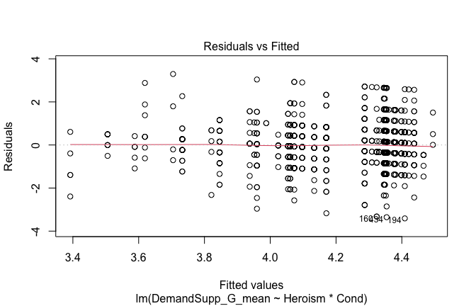

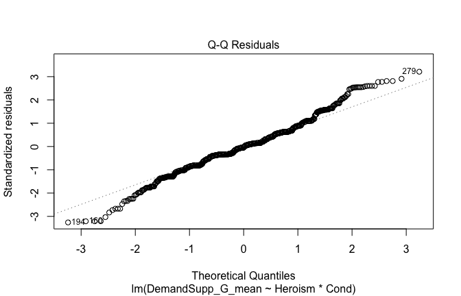
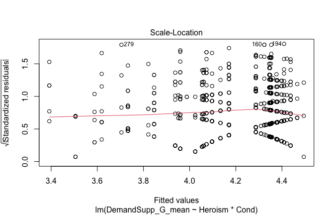
plot(mod1)

ols_plot_cooksd_bar(mod1, type = 1)

paste0("Comparison with Robust model")

## [1] "Comparison with Robust model"

models <- list("OLS (lm)" = mod1, "Robust (lmrob)" = mod1r)
modelsummary(
  models,
  statistic = c("({std.error})", "{statistic}", "p = {p.value}"),
  gof_omit  = "IC|Log.Lik",   # robust AIC comparability is iffy; omit by default
  output    = "html"
)

	OLS (lm)	Robust (lmrob)
(Intercept)	3.932	3.686
	(0.135)
	29.131
	p = <0.001
Heroism	0.052	0.095
	(0.026)
	2.043
	p = 0.041
Cond1	0.435	0.119
	(0.403)
	1.077
	p = 0.282
Cond2	0.363	0.490
	(0.229)
	1.583
	p = 0.114
Cond3	−0.460	−0.372
	(0.300)
	−1.532
	p = 0.126
Cond4	0.332	0.263
	(0.271)
	1.227
	p = 0.220
Cond5	−0.653	−0.235
	(0.270)
	−2.419
	p = 0.016
Heroism × Cond1	−0.055	−0.045
	(0.068)
	−0.817
	p = 0.414
Heroism × Cond2	−0.024	−0.068
	(0.054)
	−0.439
	p = 0.661
Heroism × Cond3	0.064	0.071
	(0.053)
	1.219
	p = 0.223
Heroism × Cond4	−0.030	−0.021
	(0.056)
	−0.538
	p = 0.591
Heroism × Cond5	0.061	0.014
	(0.051)
	1.205
	p = 0.228
Num.Obs.	840	840
R2	0.044	0.142
R2 Adj.	0.031	0.131
RMSE	1.04	1.05

fitted_vals <- fitted(mod1)

# Plot observed values against fitted values
plot(fitted_vals, scale_scores$DemandSupp_G_mean,
     xlab = "Fitted Values",
     ylab = "Observed DV",
     main = "Observed vs Fitted Values")
abline(0, 1, col = "blue", lty = 2)

paste0("####################################################")

## [1] "####################################################"

paste0("Diagnostics for Model 3: DV ~ Heroism + Occupation + Attitude")

## [1] "Diagnostics for Model 3: DV ~ Heroism + Occupation + Attitude"

paste0("####################################################")

## [1] "####################################################"

mod1 <- lm(DemandSupp_G_mean ~ Heroism  + Cond + Attitude, data = scale_scores)
mod1r <- lmrob(DemandSupp_G_mean ~ Heroism  + Cond + Attitude, data = scale_scores)
plot(mod1)

ols_plot_cooksd_bar(mod1, type = 1)

paste0("Comparison with Robust model")

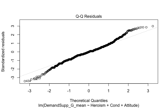
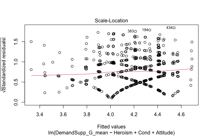
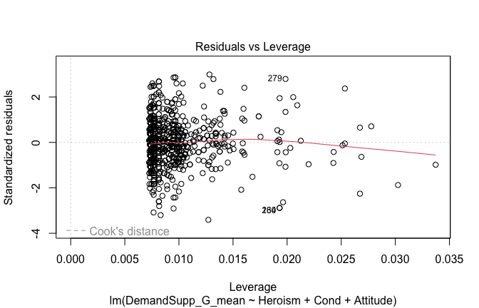
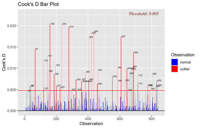
## [1] "Comparison with Robust model"

models <- list("OLS (lm)" = mod1, "Robust (lmrob)" = mod1r)
modelsummary(
  models,
  statistic = c("({std.error})", "{statistic}", "p = {p.value}"),
  gof_omit  = "IC|Log.Lik",   # robust AIC comparability is iffy; omit by default
  output    = "html"
)

	OLS (lm)	Robust (lmrob)
(Intercept)	4.221	4.258
	(0.176)	(0.185)
	23.974	23.021
	p = <0.001	p = <0.001
Heroism	−0.005	−0.016
	(0.035)	(0.037)
	−0.135	−0.425
	p = 0.893	p = 0.671
Cond1	0.056	−0.015
	(0.085)	(0.086)
	0.657	−0.168
	p = 0.511	p = 0.867
Cond2	0.333	0.345
	(0.090)	(0.077)
	3.721	4.506
	p = <0.001	p = <0.001
Cond3	−0.141	−0.097
	(0.083)	(0.087)
	−1.703	−1.117
	p = 0.089	p = 0.264
Cond4	0.178	0.196
	(0.081)	(0.069)
	2.184	2.825
	p = 0.029	p = 0.005
Cond5	−0.324	−0.320
	(0.082)	(0.080)
	−3.965	−3.979
	p = <0.001	p = <0.001
Attitude	0.156	0.160
	(0.059)	(0.063)
	2.659	2.529
	p = 0.008	p = 0.012
Num.Obs.	840	840
R2	0.048	0.056
R2 Adj.	0.040	0.048
RMSE	1.04	1.04

fitted_vals <- fitted(mod1)

# Plot observed values against fitted values
plot(fitted_vals, scale_scores$DemandSupp_G_mean,
     xlab = "Fitted Values",
     ylab = "Observed DV",
     main = "Observed vs Fitted Values")
abline(0, 1, col = "blue", lty = 2)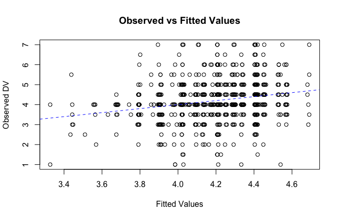

paste0("####################################################")

## [1] "####################################################"

paste0("Diagnostics for Model 4: DV ~ Heroism * Occupation + Attitude")

## [1] "Diagnostics for Model 4: DV ~ Heroism * Occupation + Attitude"

paste0("####################################################")

## [1] "####################################################"

mod1 <- lm(DemandSupp_G_mean ~ Heroism*Cond + Attitude, data = scale_scores)
mod1r <- lmrob(DemandSupp_G_mean ~ Heroism*Cond + Attitude, data = scale_scores)
plot(mod1)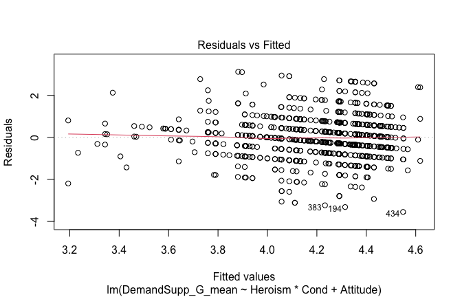

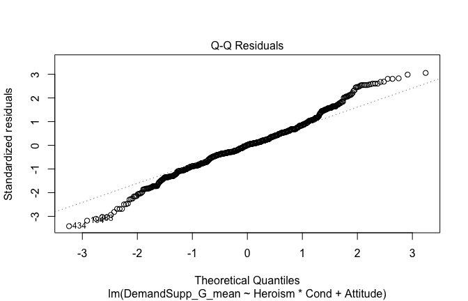
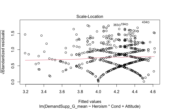
ols_plot_cooksd_bar(mod1, type = 1)

paste0("Comparison with Robust model")

## [1] "Comparison with Robust model"

models <- list("OLS (lm)" = mod1, "Robust (lmrob)" = mod1r)
modelsummary(
  models,
  statistic = c("({std.error})", "{statistic}", "p = {p.value}"),
  gof_omit  = "IC|Log.Lik",   # robust AIC comparability is iffy; omit by default
  output    = "html"
)

	OLS (lm)	Robust (lmrob)
(Intercept)	4.230	4.237
	(0.179)	(0.187)
	23.647	22.613
	p = <0.001	p = <0.001
Heroism	−0.009	−0.015
	(0.035)	(0.037)
	−0.263	−0.416
	p = 0.792	p = 0.678
Cond1	0.315	0.252
	(0.405)	(0.371)
	0.778	0.680
	p = 0.437	p = 0.497
Cond2	0.482	0.573
	(0.233)	(0.202)
	2.065	2.839
	p = 0.039	p = 0.005
Cond3	−0.504	−0.624
	(0.300)	(0.280)
	−1.680	−2.226
	p = 0.093	p = 0.026
Cond4	0.283	0.301
	(0.271)	(0.232)
	1.046	1.300
	p = 0.296	p = 0.194
Cond5	−0.516	−0.469
	(0.274)	(0.271)
	−1.882	−1.733
	p = 0.060	p = 0.083
Attitude	0.152	0.150
	(0.060)	(0.062)
	2.532	2.407
	p = 0.012	p = 0.016
Heroism × Cond1	−0.040	−0.041
	(0.068)	(0.066)
	−0.592	−0.627
	p = 0.554	p = 0.531
Heroism × Cond2	−0.041	−0.060
	(0.055)	(0.050)
	−0.748	−1.215
	p = 0.455	p = 0.225
Heroism × Cond3	0.068	0.100
	(0.052)	(0.053)
	1.289	1.878
	p = 0.198	p = 0.061
Heroism × Cond4	−0.021	−0.020
	(0.056)	(0.049)
	−0.377	−0.398
	p = 0.706	p = 0.691
Heroism × Cond5	0.040	0.033
	(0.051)	(0.055)
	0.790	0.610
	p = 0.430	p = 0.542
Num.Obs.	840	840
R2	0.051	0.062
R2 Adj.	0.037	0.048
RMSE	1.04	1.04

fitted_vals <- fitted(mod1)

# Plot observed values against fitted values
plot(fitted_vals, scale_scores$DemandSupp_G_mean,
     xlab = "Fitted Values",
     ylab = "Observed DV",
     main = "Observed vs Fitted Values")
abline(0, 1, col = "blue", lty = 2)

paste0("####################################################")

## [1] "####################################################"

paste0("REPORTS for each model (please ignore the eta squares, they are way off")

## [1] "REPORTS for each model (please ignore the eta squares, they are way off"

paste0("####################################################")

## [1] "####################################################"

paste0("MODEL 1: DemandSupp_G_mean ~ Heroism")

## [1] "MODEL 1: DemandSupp_G_mean ~ Heroism"

report(Anova(mod1 <- lm(DemandSupp_G_mean ~ Heroism  + Cond, data = scale_scores), type = "III"))

## The ANOVA suggests that:
## 
##   - The main effect of Heroism is statistically significant and very small (F(1,
## 833) = 5.99, p = 0.015; Eta2 (partial) = 7.14e-03, 95% CI [7.53e-04, 1.00])
##   - The main effect of Cond is statistically significant and small (F(5, 833) =
## 6.48, p < .001; Eta2 (partial) = 0.04, 95% CI [0.02, 1.00])
## 
## Effect sizes were labelled following Field's (2013) recommendations.

paste0("MODEL 2: DemandSupp_G_mean ~ Heroism * Cond")

## [1] "MODEL 2: DemandSupp_G_mean ~ Heroism * Cond"

report(Anova(mod2 <- lm(DemandSupp_G_mean ~ Heroism * Cond, data = scale_scores), type = "III"))

## Type 3 ANOVAs only give sensible and informative results when covariates
##   are mean-centered and factors are coded with orthogonal contrasts (such
##   as those produced by `contr.sum`, `contr.poly`, or `contr.helmert`, but
##   *not* by the default `contr.treatment`).

## The ANOVA suggests that:
## 
##   - The main effect of Heroism is statistically significant and very small (F(1,
## 828) = 4.18, p = 0.041; Eta2 (partial) = 5.02e-03, 95% CI [1.03e-04, 1.00])
##   - The main effect of Cond is statistically significant and small (F(5, 828) =
## 2.38, p = 0.037; Eta2 (partial) = 0.01, 95% CI [4.39e-04, 1.00])
##   - The interaction between Heroism and Cond is statistically not significant and
## very small (F(5, 828) = 0.69, p = 0.628; Eta2 (partial) = 4.17e-03, 95% CI
## [0.00, 1.00])
## 
## Effect sizes were labelled following Field's (2013) recommendations.

paste0("MODEL 3: DemandSupp_G_mean ~ Heroism +scale(Attitude)")

## [1] "MODEL 3: DemandSupp_G_mean ~ Heroism +scale(Attitude)"

report(Anova(mod3 <- lm(DemandSupp_G_mean ~ Heroism   + Cond +scale(Attitude) , data = scale_scores), type = "III"))

## The ANOVA suggests that:
## 
##   - The main effect of Heroism is statistically not significant and very small
## (F(1, 832) = 0.02, p = 0.893; Eta2 (partial) = 2.20e-05, 95% CI [0.00, 1.00])
##   - The main effect of Cond is statistically significant and small (F(5, 832) =
## 6.58, p < .001; Eta2 (partial) = 0.04, 95% CI [0.02, 1.00])
##   - The main effect of scale(Attitude) is statistically significant and very
## small (F(1, 832) = 7.07, p = 0.008; Eta2 (partial) = 8.42e-03, 95% CI
## [1.22e-03, 1.00])
## 
## Effect sizes were labelled following Field's (2013) recommendations.

paste0("MODEL 4: DemandSupp_G_mean ~ Heroism * Cond + scale(Attitude)")

## [1] "MODEL 4: DemandSupp_G_mean ~ Heroism * Cond + scale(Attitude)"

report(Anova(mod4 <-lm(DemandSupp_G_mean ~ Heroism * Cond + scale(Attitude), data = scale_scores), type = "III"))

## Type 3 ANOVAs only give sensible and informative results when covariates
##   are mean-centered and factors are coded with orthogonal contrasts (such
##   as those produced by `contr.sum`, `contr.poly`, or `contr.helmert`, but
##   *not* by the default `contr.treatment`).

## The ANOVA suggests that:
## 
##   - The main effect of Heroism is statistically not significant and very small
## (F(1, 827) = 0.07, p = 0.792; Eta2 (partial) = 8.38e-05, 95% CI [0.00, 1.00])
##   - The main effect of Cond is statistically significant and small (F(5, 827) =
## 2.30, p = 0.043; Eta2 (partial) = 0.01, 95% CI [2.16e-04, 1.00])
##   - The main effect of scale(Attitude) is statistically significant and very
## small (F(1, 827) = 6.41, p = 0.012; Eta2 (partial) = 7.69e-03, 95% CI
## [9.35e-04, 1.00])
##   - The interaction between Heroism and Cond is statistically not significant and
## very small (F(5, 827) = 0.57, p = 0.723; Eta2 (partial) = 3.44e-03, 95% CI
## [0.00, 1.00])
## 
## Effect sizes were labelled following Field's (2013) recommendations.

paste0("Model Comparison: assessing the importance of attitude - not accounting for occupations")

## [1] "Model Comparison: assessing the importance of attitude - not accounting for occupations"

anova(mod1, mod3)

paste0("Model Comparison: assessing the importance of attitude - accounting for occupations")

## [1] "Model Comparison: assessing the importance of attitude - accounting for occupations"

anova(mod2, mod4)

ggplot(scale_scores, aes(y = DemandSupp_G_mean, x = Heroism)) +
  # 1) points colored by Cond
  geom_point(aes(color = Cond),
             size = 2.7, alpha = 0.7) +
  
  # 2) ONE global lm line (group = 1 prevents one line per Cond)
  stat_smooth(method = "lm", se = TRUE,
              aes(group = 1),
              color = "black", linewidth = 1) +
  
  # Nice, accessible palette (works well with >3 groups)
  scale_color_brewer(palette = "Set2") +
  
  labs(
    y = "Support for demands (G)",
    x = "Heroism",
    color = "Occupation",
    title = "Heroism vs. Support for demands (G), colored by Occupation",
    subtitle = "Points are participants; black line is overall linear fit with 95% CI"
  ) +
  theme_minimal(base_size = 12) +
  theme(
    legend.position = "right",
    panel.grid.minor = element_blank()
  )

## `geom_smooth()` using formula = 'y ~ x'

ggplot(scale_scores, aes(x = Heroism, y = DemandSupp_G_mean, color = Cond)) +
  # points colored by condition
  geom_point(size = 2.7, alpha = 0.7) +
  # ONE lm line PER condition (because color is mapped here)
  stat_smooth(method = "lm", se = FALSE, linewidth = 1, fullrange = TRUE) +
  scale_color_brewer(palette = "Set2") +
  labs(
    y = "Support for demands (G)",
    x = "Heroism",
    color = "Occupation",
    title = "Heroism vs. Support for demands (G) with per-Occupation linear fits"
  ) +
  theme_minimal(base_size = 12) +
  theme(legend.position = "right", panel.grid.minor = element_blank())

## `geom_smooth()` using formula = 'y ~ x'

Note that there are two items here: 1) The government, and not the workers, are justified to demand changes ; and 2) the workers, and not the government are justified to demand changes. In this analysis - item 1 was reversed, so that overall score reflects support for workers (rather than government) demanding changes. Nevertheless – as we have seen in the psychometric analyses of the scale: the internal consistency is low, which might be explained by the fact that the two items are not mutually exclusive.

Overall, very small effect sizes for this measure of general support for workers demands - all eta2 < .01. It is not of interest, despite significance. Moreover, effects run in the opposite direction to our predictions, see table:

Model 1: “~Heroism + Occupation”

# =========================
# OLD MODELS (Heroism)
# =========================
m1_H <- lm(DemandSupp_G_mean ~ Heroism + Occupation, data = scale_scores)
m2_H <- lm(DemandSupp_G_mean ~ Heroism * Occupation, data = scale_scores)
m3_H <- lm(DemandSupp_G_mean ~ Heroism + Occupation + Attitude, data = scale_scores)
m4_H <- lm(DemandSupp_G_mean ~ Heroism * Occupation + Attitude, data = scale_scores)

tidy_type3(m1_H, "~Heroism + Cond")

~Heroism + Cond
	Term	df1	df2	F	p	eta2p
Heroism	Heroism	1	833	5.99	= 0.015	0.007
Occupation	Occupation	5	833	6.48	< .001	0.037

# =========================
# NEW MODELS (Danger & Help)
# =========================

Model 2: “~Heroism * Occupation”

tidy_type3(m2_H, "~Heroism * Cond")

~Heroism * Cond
	Term	df1	df2	F	p	eta2p
Heroism	Heroism	1	828	4.18	= 0.041	0.005
Occupation	Occupation	5	828	2.38	= 0.037	0.014
Heroism:Occupation	Heroism:Occupation	5	828	0.69	= 0.628	0.004

Model 3: “~Heroism + Occupation + Attitude”

tidy_type3(m3_H, "~Heroism + Occupation + Attitude")

~Heroism + Occupation + Attitude
	Term	df1	df2	F	p	eta2p
Heroism	Heroism	1	832	0.02	= 0.893	0.000
Occupation	Occupation	5	832	6.58	< .001	0.038
Attitude	Attitude	1	832	7.07	= 0.008	0.008

Model 4: “~Heroism * Occupation + Attitude”

tidy_type3(m4_H, "~Heroism * Occupation + Attitude")

~Heroism * Occupation + Attitude
	Term	df1	df2	F	p	eta2p
Heroism	Heroism	1	827	0.07	= 0.792	0.000
Occupation	Occupation	5	827	2.30	= 0.043	0.014
Attitude	Attitude	1	827	6.41	= 0.012	0.008
Heroism:Occupation	Heroism:Occupation	5	827	0.57	= 0.723	0.003

Comparison of main predictors across models

# Use orthogonal contrasts; keeps your "Heroism main effect" interpretable with Cond in the model
old_contr <- options(contrasts = c("contr.sum", "contr.poly"))

# Helper to extract the main effect of "Heroism" from a car::Anova table
extract_heroism <- function(mod, model_label) {
  a <- car::Anova(mod, type = "III")

  # Coerce to data.frame with rownames preserved
  tab <- as.data.frame(a)
  tab$Term <- rownames(tab)

  # Standard column names across R versions
  # (car::Anova uses these names for lm/glm type=III)
  # Columns: "Sum Sq", "Df", "F value", "Pr(>F)"
  names(tab) <- sub(" ", "_", names(tab))  # make names safe: "Sum_Sq", "F_value", etc.

  # Pull rows we need
  hero <- tab %>% filter(Term == "Heroism")
  resid <- tab %>% filter(Term == "Residuals")

  # Safety checks (in case of name variants)
  stopifnot(nrow(hero) == 1, nrow(resid) == 1)

  # Partial eta^2 = SS_effect / (SS_effect + SS_residual)
  eta_p2 <- hero$Sum_Sq / (hero$Sum_Sq + resid$Sum_Sq)

  # Format p nicely (APA-ish)
  p_fmt <- ifelse(hero$`Pr(>F)` < .001, "< .001",
                  sprintf("= %.3f", hero$`Pr(>F)`))

  dplyr::tibble(
    Model = model_label,
    Outcome = "DemandSupp_G_mean",
    Predictor = "Heroism",
    df1 = hero$Df,
    df2 = resid$Df,
    F = hero$F_value,
    p = p_fmt,
    eta2p = eta_p2
  )
}

# ----- Fit the four models -----
mod1 <- lm(DemandSupp_G_mean ~ Heroism + Cond, data = scale_scores)
mod2 <- lm(DemandSupp_G_mean ~ Heroism * Cond, data = scale_scores)
mod3 <- lm(DemandSupp_G_mean ~ Heroism + Cond + scale(Attitude), data = scale_scores)
mod4 <- lm(DemandSupp_G_mean ~ Heroism * Cond + scale(Attitude), data = scale_scores)

# ----- Build the summary table -----
tbl <- bind_rows(
  extract_heroism(mod1, "~ Heroism + Cond"),
  extract_heroism(mod2, "~ Heroism * Occupation"),
  extract_heroism(mod3, "~ Heroism + Cond + Attitude"),
  extract_heroism(mod4, "~ Heroism * Occupation + Attitude")
  ) %>%
  # Nice number formatting for F and eta^2p
  mutate(
    F = round(F, 2),
    eta2p = round(eta2p, 3)
  )

# ----- Print as HTML-friendly table -----
# Build the table first
tbl_kbl <- tbl %>%
  kable("html",
        caption = "Main effect of Heroism across models (Type-III ANOVA): F, p, partial η²",
        align = "lllrrrcr")
# Add a footnote in a version-robust way
if ("footnote" %in% getNamespaceExports("kableExtra")) {
  tbl_kbl <- tbl_kbl %>%
    kableExtra::footnote(
      general = "Type-III sums of squares with sum contrasts. Partial η² = SS_effect / (SS_effect + SS_residual). p values are APA-style.",
      general_title = ""
    )
} else {
  tbl_kbl <- tbl_kbl %>%
    kableExtra::add_footnote(
      label = "Type-III sums of squares with sum contrasts. Partial η² = SS_effect / (SS_effect + SS_residual). p values are APA-style.",
      notation = "none"
    )
}

tbl_kbl

Main effect of Heroism across models (Type-III ANOVA): F, p, partial η²
Model	Outcome	Predictor	df1	df2	F	p	eta2p
~ Heroism + Cond	DemandSupp_G_mean	Heroism	1	833	5.99	= 0.015	0.007
~ Heroism * Occupation	DemandSupp_G_mean	Heroism	1	828	4.18	= 0.041	0.005
~ Heroism + Cond + Attitude	DemandSupp_G_mean	Heroism	1	832	0.02	= 0.893	0.000
~ Heroism * Occupation + Attitude	DemandSupp_G_mean	Heroism	1	827	0.07	= 0.792	0.000
Type-III sums of squares with sum contrasts. Partial η² = SS_effect / (SS_effect + SS_residual). p values are APA-style.

Specific level

Journalists should protest more for the rights they deserve

Toggle details of the models diagnostics and outlier analyses

Below, you’ll find model diagnostics (QQ plot, fitted vs residuals, linearity), Outliers analysis, and more details on the output

[NOTE THAT EFFECT SIZES REPORTED IN THE REPORT COMMANDS BELOW SHOULD NOT BE TRUSTED]

paste0("####################################################")

## [1] "####################################################"

paste0("Diagnostics for Model 1: DV ~ Heroism + Occupation")

## [1] "Diagnostics for Model 1: DV ~ Heroism + Occupation"

paste0("####################################################")

## [1] "####################################################"

mod1 <- lm(DemandSupp_S_mean ~ Heroism  + Cond, data = scale_scores)
mod1r <- lmrob(DemandSupp_S_mean ~ Heroism  + Cond, data = scale_scores)
plot(mod1)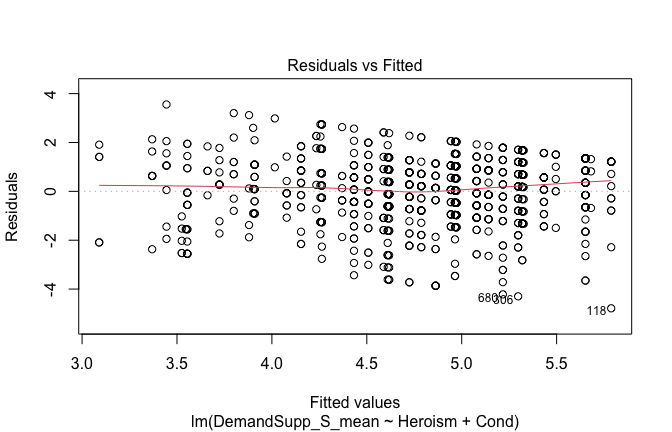

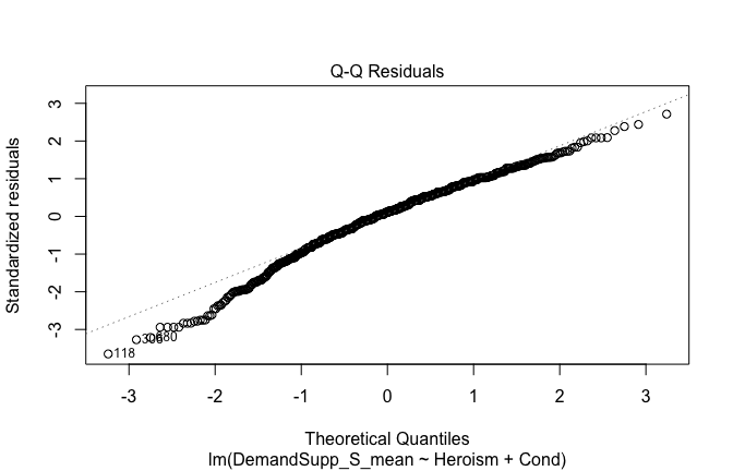
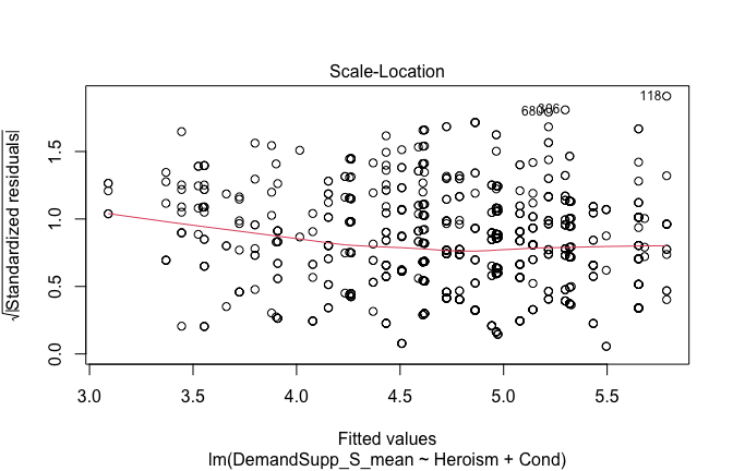
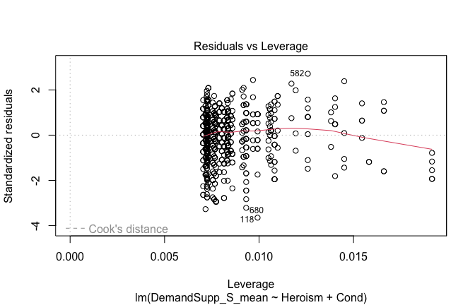
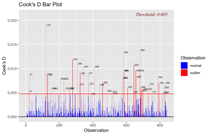
ols_plot_cooksd_bar(mod1, type = 1)

paste0("Comparison with Robust model")

## [1] "Comparison with Robust model"

models <- list("OLS (lm)" = mod1, "Robust (lmrob)" = mod1r)
modelsummary(
  models,
  statistic = c("({std.error})", "{statistic}", "p = {p.value}"),
  gof_omit  = "IC|Log.Lik",   # robust AIC comparability is iffy; omit by default
  output    = "html"
)

	OLS (lm)	Robust (lmrob)
(Intercept)	3.044	2.948
	(0.161)	(0.207)
	18.957	14.221
	p = <0.001	p = <0.001
Heroism	0.354	0.393
	(0.031)	(0.039)
	11.334	10.097
	p = <0.001	p = <0.001
Cond1	−0.206	−0.250
	(0.106)	(0.110)
	−1.944	−2.273
	p = 0.052	p = 0.023
Cond2	0.156	0.164
	(0.110)	(0.112)
	1.410	1.464
	p = 0.159	p = 0.144
Cond3	0.126	0.088
	(0.104)	(0.112)
	1.218	0.788
	p = 0.224	p = 0.431
Cond4	−0.030	−0.067
	(0.102)	(0.092)
	−0.289	−0.730
	p = 0.773	p = 0.466
Cond5	−0.309	−0.195
	(0.102)	(0.115)
	−3.012	−1.690
	p = 0.003	p = 0.091
Num.Obs.	840	840
R2	0.163	0.202
R2 Adj.	0.157	0.197
RMSE	1.31	1.32

fitted_vals <- fitted(mod1)

# Plot observed values against fitted values
plot(fitted_vals, scale_scores$DemandSupp_S_mean,
     xlab = "Fitted Values",
     ylab = "Observed DV",
     main = "Observed vs Fitted Values")
abline(0, 1, col = "blue", lty = 2)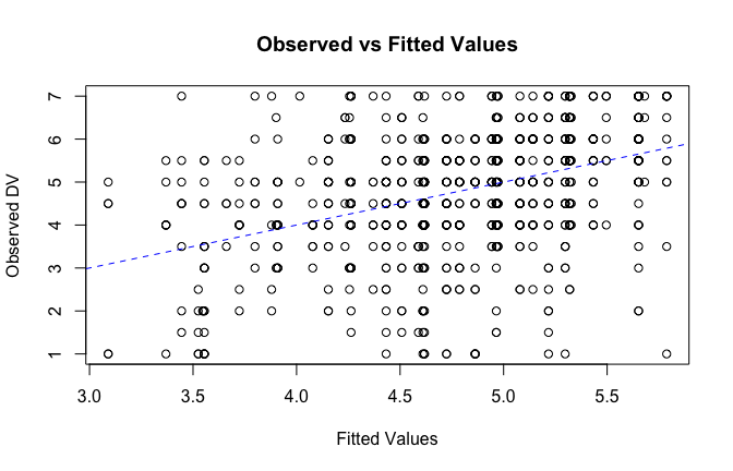

paste0("####################################################")

## [1] "####################################################"

paste0("Diagnostics for Model 2: DV ~ Heroism * Occupation")

## [1] "Diagnostics for Model 2: DV ~ Heroism * Occupation"

paste0("####################################################")

## [1] "####################################################"

mod1 <- lm(DemandSupp_S_mean ~ Heroism  * Cond, data = scale_scores)
mod1r <- lmrob(DemandSupp_S_mean ~ Heroism  * Cond, data = scale_scores)
plot(mod1)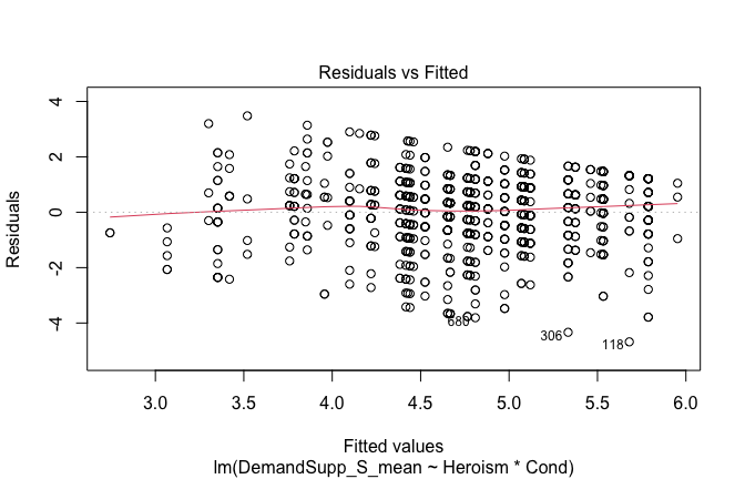

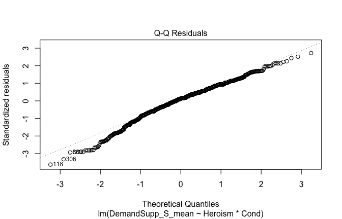
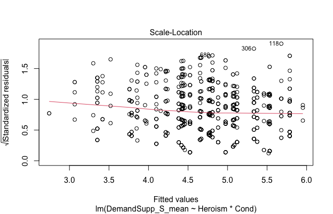
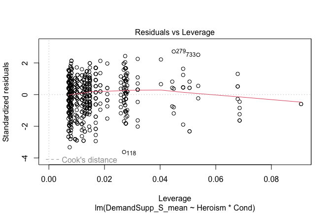
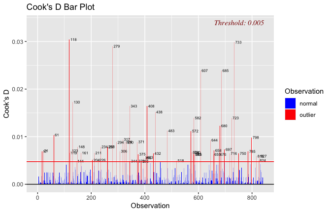
ols_plot_cooksd_bar(mod1, type = 1)

paste0("Comparison with Robust model")

## [1] "Comparison with Robust model"

models <- list("OLS (lm)" = mod1, "Robust (lmrob)" = mod1r)
modelsummary(
  models,
  statistic = c("({std.error})", "{statistic}", "p = {p.value}"),
  gof_omit  = "IC|Log.Lik",   # robust AIC comparability is iffy; omit by default
  output    = "html"
)

	OLS (lm)	Robust (lmrob)
(Intercept)	2.933	2.798
	(0.168)	(0.192)
	17.438	14.558
	p = <0.001	p = <0.001
Heroism	0.372	0.413
	(0.032)	(0.035)
	11.645	11.679
	p = <0.001	p = <0.001
Cond1	−1.305	−1.545
	(0.503)	(0.557)
	−2.596	−2.773
	p = 0.010	p = 0.006
Cond2	−0.014	0.179
	(0.286)	(0.328)
	−0.048	0.547
	p = 0.961	p = 0.584
Cond3	−0.319	−0.660
	(0.374)	(0.485)
	−0.854	−1.359
	p = 0.394	p = 0.175
Cond4	0.146	0.369
	(0.338)	(0.335)
	0.432	1.102
	p = 0.666	p = 0.271
Cond5	0.881	1.038
	(0.336)	(0.441)
	2.620	2.354
	p = 0.009	p = 0.019
Heroism × Cond1	0.186	0.220
	(0.084)	(0.089)
	2.200	2.472
	p = 0.028	p = 0.014
Heroism × Cond2	0.061	0.018
	(0.068)	(0.073)
	0.905	0.247
	p = 0.366	p = 0.805
Heroism × Cond3	0.081	0.136
	(0.066)	(0.079)
	1.242	1.711
	p = 0.214	p = 0.088
Heroism × Cond4	−0.032	−0.082
	(0.070)	(0.068)
	−0.457	−1.210
	p = 0.648	p = 0.227
Heroism × Cond5	−0.230	−0.231
	(0.063)	(0.084)
	−3.639	−2.732
	p = <0.001	p = 0.006
Num.Obs.	840	840
R2	0.181	0.231
R2 Adj.	0.170	0.220
RMSE	1.30	1.31

fitted_vals <- fitted(mod1)

# Plot observed values against fitted values
plot(fitted_vals, scale_scores$DemandSupp_S_mean,
     xlab = "Fitted Values",
     ylab = "Observed DV",
     main = "Observed vs Fitted Values")
abline(0, 1, col = "blue", lty = 2)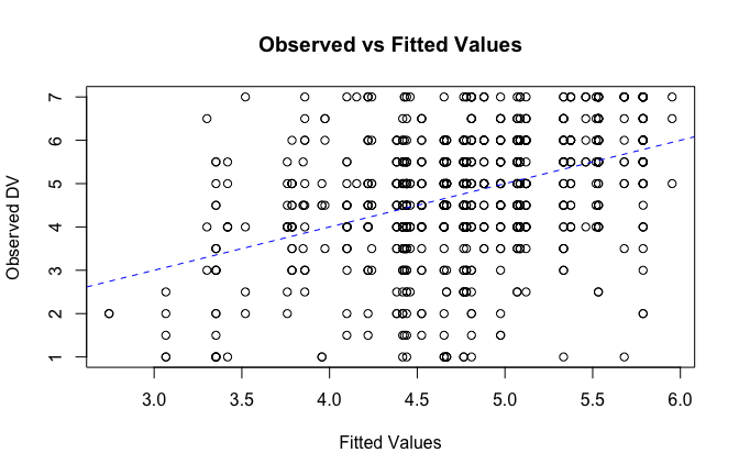

paste0("####################################################")

## [1] "####################################################"

paste0("Diagnostics for Model 3: DV ~ Heroism + Occupation + Attitude")

## [1] "Diagnostics for Model 3: DV ~ Heroism + Occupation + Attitude"

paste0("####################################################")

## [1] "####################################################"

mod1 <- lm(DemandSupp_S_mean ~ Heroism  + Cond + Attitude, data = scale_scores)
mod1r <- lmrob(DemandSupp_S_mean ~ Heroism  + Cond + Attitude, data = scale_scores)
plot(mod1)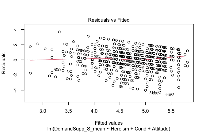

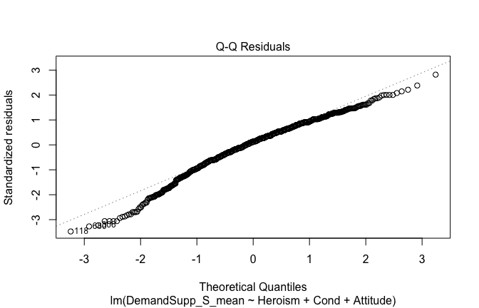
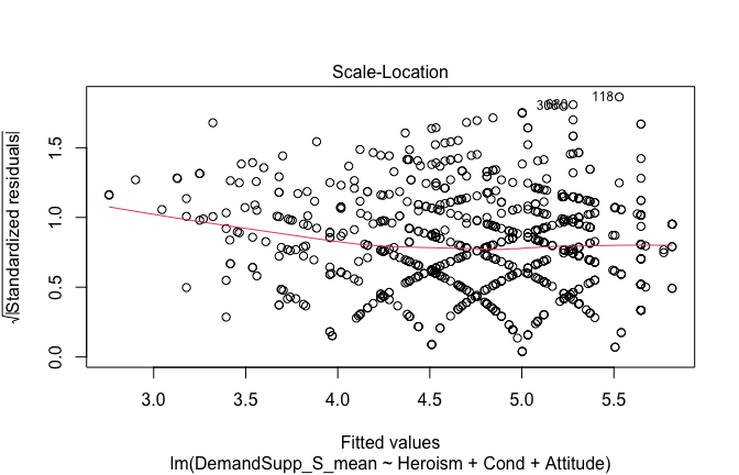
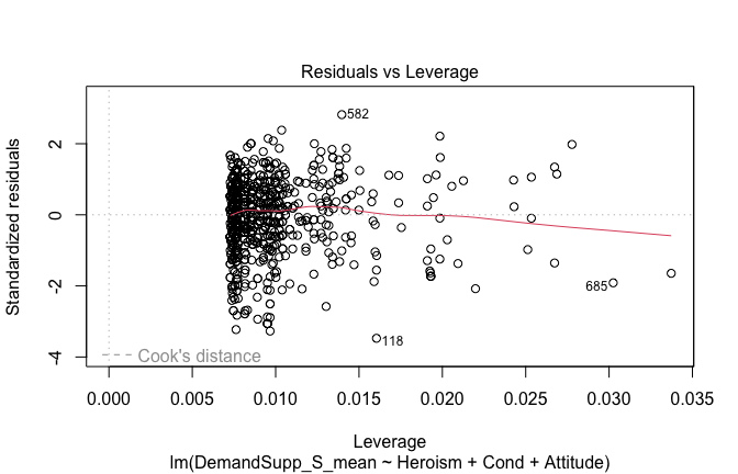
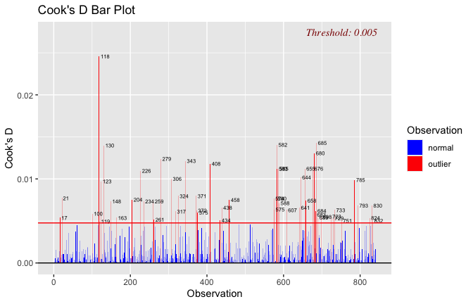
ols_plot_cooksd_bar(mod1, type = 1)

paste0("Comparison with Robust model")

## [1] "Comparison with Robust model"

models <- list("OLS (lm)" = mod1, "Robust (lmrob)" = mod1r)
modelsummary(
  models,
  statistic = c("({std.error})", "{statistic}", "p = {p.value}"),
  gof_omit  = "IC|Log.Lik",   # robust AIC comparability is iffy; omit by default
  output    = "html"
)

	OLS (lm)	Robust (lmrob)
(Intercept)	3.429	3.469
	(0.221)	(0.286)
	15.485	12.114
	p = <0.001	p = <0.001
Heroism	0.276	0.289
	(0.044)	(0.055)
	6.285	5.284
	p = <0.001	p = <0.001
Cond1	−0.246	−0.291
	(0.107)	(0.109)
	−2.296	−2.673
	p = 0.022	p = 0.008
Cond2	0.216	0.223
	(0.113)	(0.110)
	1.918	2.020
	p = 0.055	p = 0.044
Cond3	0.092	0.043
	(0.104)	(0.109)
	0.884	0.395
	p = 0.377	p = 0.693
Cond4	−0.048	−0.095
	(0.102)	(0.091)
	−0.471	−1.045
	p = 0.637	p = 0.296
Cond5	−0.276	−0.130
	(0.103)	(0.121)
	−2.684	−1.075
	p = 0.007	p = 0.282
Attitude	0.186	0.242
	(0.074)	(0.090)
	2.514	2.697
	p = 0.012	p = 0.007
Num.Obs.	840	840
R2	0.169	0.215
R2 Adj.	0.162	0.208
RMSE	1.31	1.32

fitted_vals <- fitted(mod1)

# Plot observed values against fitted values
plot(fitted_vals, scale_scores$DemandSupp_S_mean,
     xlab = "Fitted Values",
     ylab = "Observed DV",
     main = "Observed vs Fitted Values")
abline(0, 1, col = "blue", lty = 2)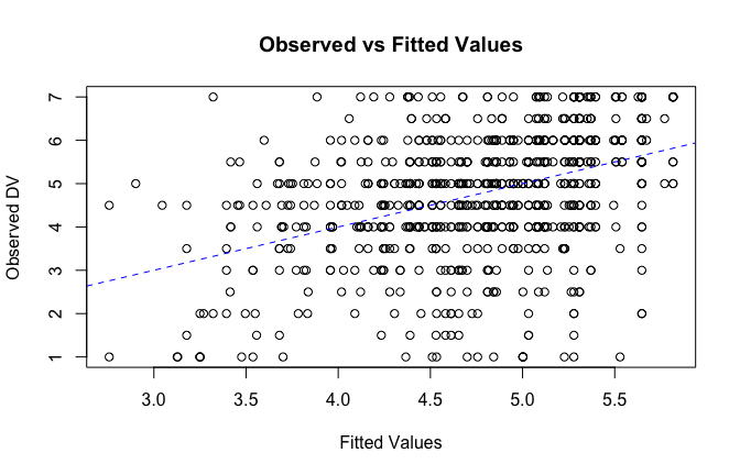

paste0("####################################################")

## [1] "####################################################"

paste0("Diagnostics for Model 4: DV ~ Heroism * Occupation + Attitude")

## [1] "Diagnostics for Model 4: DV ~ Heroism * Occupation + Attitude"

paste0("####################################################")

## [1] "####################################################"

mod1 <- lm(DemandSupp_S_mean ~ Heroism*Cond + Attitude, data = scale_scores)
mod1r <- lmrob(DemandSupp_S_mean ~ Heroism*Cond + Attitude, data = scale_scores)
plot(mod1)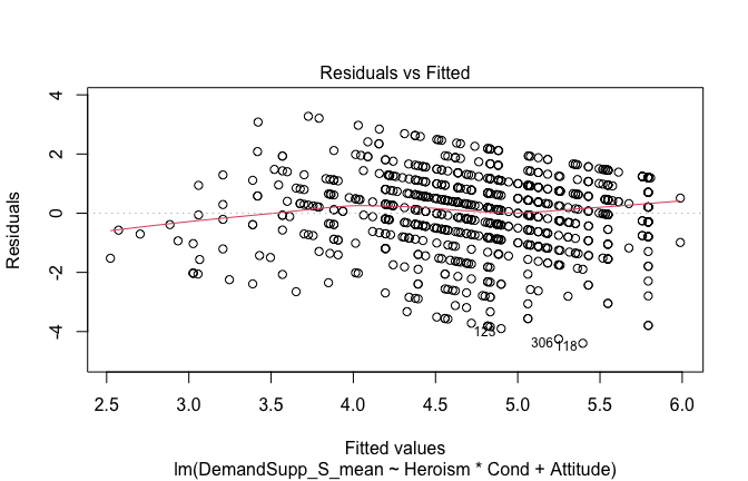

ols_plot_cooksd_bar(mod1, type = 1)

paste0("Comparison with Robust model")

## [1] "Comparison with Robust model"

models <- list("OLS (lm)" = mod1, "Robust (lmrob)" = mod1r)
modelsummary(
  models,
  statistic = c("({std.error})", "{statistic}", "p = {p.value}"),
  gof_omit  = "IC|Log.Lik",   # robust AIC comparability is iffy; omit by default
  output    = "html"
)

	OLS (lm)	Robust (lmrob)
(Intercept)	3.391	3.421
	(0.222)	(0.285)
	15.240	12.006
	p = <0.001	p = <0.001
Heroism	0.277	0.288
	(0.044)	(0.054)
	6.319	5.388
	p = <0.001	p = <0.001
Cond1	−1.489	−1.710
	(0.504)	(0.565)
	−2.957	−3.025
	p = 0.003	p = 0.003
Cond2	0.168	0.315
	(0.290)	(0.304)
	0.580	1.036
	p = 0.562	p = 0.301
Cond3	−0.387	−0.687
	(0.373)	(0.452)
	−1.036	−1.520
	p = 0.300	p = 0.129
Cond4	0.070	0.208
	(0.337)	(0.320)
	0.208	0.652
	p = 0.835	p = 0.515
Cond5	1.091	1.306
	(0.341)	(0.442)
	3.196	2.955
	p = 0.001	p = 0.003
Attitude	0.234	0.288
	(0.075)	(0.088)
	3.122	3.285
	p = 0.002	p = 0.001
Heroism × Cond1	0.209	0.240
	(0.084)	(0.090)
	2.480	2.665
	p = 0.013	p = 0.008
Heroism × Cond2	0.035	0.001
	(0.068)	(0.069)
	0.519	0.007
	p = 0.604	p = 0.994
Heroism × Cond3	0.087	0.133
	(0.065)	(0.075)
	1.330	1.784
	p = 0.184	p = 0.075
Heroism × Cond4	−0.018	−0.054
	(0.069)	(0.065)
	−0.259	−0.831
	p = 0.796	p = 0.406
Heroism × Cond5	−0.262	−0.267
	(0.064)	(0.083)
	−4.109	−3.200
	p = <0.001	p = 0.001
Num.Obs.	840	840
R2	0.191	0.244
R2 Adj.	0.179	0.233
RMSE	1.29	1.30

fitted_vals <- fitted(mod1)

# Plot observed values against fitted values
plot(fitted_vals, scale_scores$DemandSupp_S_mean,
     xlab = "Fitted Values",
     ylab = "Observed DV",
     main = "Observed vs Fitted Values")
abline(0, 1, col = "blue", lty = 2)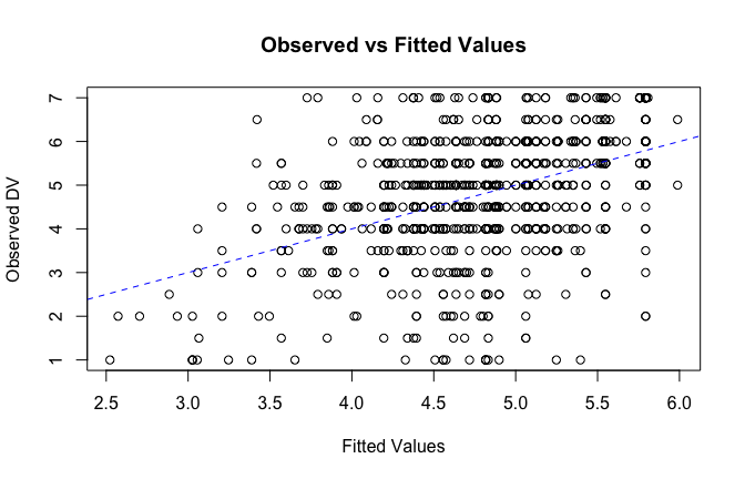

paste0("####################################################")

## [1] "####################################################"

paste0("REPORTS for each model (please ignore the eta squares, they are way off")

## [1] "REPORTS for each model (please ignore the eta squares, they are way off"

paste0("####################################################")

## [1] "####################################################"

paste0("MODEL 1: DemandSupp_S_mean ~ Heroism")

## [1] "MODEL 1: DemandSupp_S_mean ~ Heroism"

report(Anova(mod1 <- lm(DemandSupp_S_mean ~ Heroism  + Cond, data = scale_scores), type = "III"))

## The ANOVA suggests that:
## 
##   - The main effect of Heroism is statistically significant and medium (F(1, 833)
## = 128.46, p < .001; Eta2 (partial) = 0.13, 95% CI [0.10, 1.00])
##   - The main effect of Cond is statistically significant and small (F(5, 833) =
## 3.80, p = 0.002; Eta2 (partial) = 0.02, 95% CI [4.98e-03, 1.00])
## 
## Effect sizes were labelled following Field's (2013) recommendations.

paste0("MODEL 2: DemandSupp_S_mean ~ Heroism * Cond")

## [1] "MODEL 2: DemandSupp_S_mean ~ Heroism * Cond"

report(Anova(mod2 <- lm(DemandSupp_S_mean ~ Heroism * Cond, data = scale_scores), type = "III"))

## Type 3 ANOVAs only give sensible and informative results when covariates
##   are mean-centered and factors are coded with orthogonal contrasts (such
##   as those produced by `contr.sum`, `contr.poly`, or `contr.helmert`, but
##   *not* by the default `contr.treatment`).

## The ANOVA suggests that:
## 
##   - The main effect of Heroism is statistically significant and large (F(1, 828)
## = 135.61, p < .001; Eta2 (partial) = 0.14, 95% CI [0.11, 1.00])
##   - The main effect of Cond is statistically significant and small (F(5, 828) =
## 2.66, p = 0.021; Eta2 (partial) = 0.02, 95% CI [1.26e-03, 1.00])
##   - The interaction between Heroism and Cond is statistically significant and
## small (F(5, 828) = 3.63, p = 0.003; Eta2 (partial) = 0.02, 95% CI [4.41e-03,
## 1.00])
## 
## Effect sizes were labelled following Field's (2013) recommendations.

paste0("MODEL 3: DemandSupp_S_mean ~ Heroism +scale(Attitude)")

## [1] "MODEL 3: DemandSupp_S_mean ~ Heroism +scale(Attitude)"

report(Anova(mod3 <- lm(DemandSupp_S_mean ~ Heroism   + Cond +scale(Attitude) , data = scale_scores), type = "III"))

## The ANOVA suggests that:
## 
##   - The main effect of Heroism is statistically significant and small (F(1, 832)
## = 39.50, p < .001; Eta2 (partial) = 0.05, 95% CI [0.03, 1.00])
##   - The main effect of Cond is statistically significant and small (F(5, 832) =
## 3.94, p = 0.002; Eta2 (partial) = 0.02, 95% CI [5.49e-03, 1.00])
##   - The main effect of scale(Attitude) is statistically significant and very
## small (F(1, 832) = 6.32, p = 0.012; Eta2 (partial) = 7.54e-03, 95% CI
## [8.91e-04, 1.00])
## 
## Effect sizes were labelled following Field's (2013) recommendations.

paste0("MODEL 4: DemandSupp_S_mean ~ Heroism * Cond + scale(Attitude)")

## [1] "MODEL 4: DemandSupp_S_mean ~ Heroism * Cond + scale(Attitude)"

report(Anova(mod4 <-lm(DemandSupp_S_mean ~ Heroism * Cond + scale(Attitude), data = scale_scores), type = "III"))

## Type 3 ANOVAs only give sensible and informative results when covariates
##   are mean-centered and factors are coded with orthogonal contrasts (such
##   as those produced by `contr.sum`, `contr.poly`, or `contr.helmert`, but
##   *not* by the default `contr.treatment`).

## The ANOVA suggests that:
## 
##   - The main effect of Heroism is statistically significant and small (F(1, 827)
## = 39.92, p < .001; Eta2 (partial) = 0.05, 95% CI [0.03, 1.00])
##   - The main effect of Cond is statistically significant and small (F(5, 827) =
## 3.42, p = 0.005; Eta2 (partial) = 0.02, 95% CI [3.70e-03, 1.00])
##   - The main effect of scale(Attitude) is statistically significant and small
## (F(1, 827) = 9.75, p = 0.002; Eta2 (partial) = 0.01, 95% CI [2.61e-03, 1.00])
##   - The interaction between Heroism and Cond is statistically significant and
## small (F(5, 827) = 4.33, p < .001; Eta2 (partial) = 0.03, 95% CI [6.93e-03,
## 1.00])
## 
## Effect sizes were labelled following Field's (2013) recommendations.

paste0("Model Comparison: assessing the importance of attitude - not accounting for occupations")

## [1] "Model Comparison: assessing the importance of attitude - not accounting for occupations"

anova(mod1, mod3)

paste0("Model Comparison: assessing the importance of attitude - accounting for occupations")

## [1] "Model Comparison: assessing the importance of attitude - accounting for occupations"

anova(mod2, mod4)

ggplot(scale_scores, aes(y = DemandSupp_S_mean, x = Heroism)) +
  # 1) points colored by Cond
  geom_point(aes(color = Cond),
             size = 2.7, alpha = 0.7) +
  
  # 2) ONE global lm line (group = 1 prevents one line per Cond)
  stat_smooth(method = "lm", se = TRUE,
              aes(group = 1),
              color = "black", linewidth = 1) +
  
  # Nice, accessible palette (works well with >3 groups)
  scale_color_brewer(palette = "Set2") +
  
  labs(
    y = "Support for demands (S)",
    x = "Heroism",
    color = "Occupation",
    title = "Heroism vs. Support for demands (S), colored by Occupation",
    subtitle = "Points are participants; black line is overall linear fit with 95% CI"
  ) +
  theme_minimal(base_size = 12) +
  theme(
    legend.position = "right",
    panel.grid.minor = element_blank()
  )

## `geom_smooth()` using formula = 'y ~ x'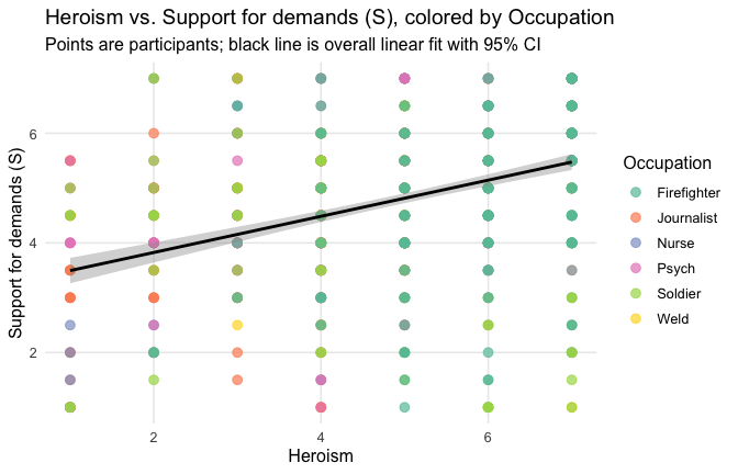

ggplot(scale_scores, aes(y = DemandSupp_S_mean, x = Heroism, color = Cond)) +
  # points colored by condition
  geom_point(size = 2.7, alpha = 0.7) +
  # ONE lm line PER condition (because color is mapped here)
  stat_smooth(method = "lm", se = FALSE, linewidth = 1, fullrange = TRUE) +
  scale_color_brewer(palette = "Set2") +
  labs(
    y = "Support for demands (S) ",
    x = "Heroism",
    color = "Occupation",
    title = "Heroism vs. Support for demands (S) with per-Occupation linear fits"
  ) +
  theme_minimal(base_size = 12) +
  theme(legend.position = "right", panel.grid.minor = element_blank())

## `geom_smooth()` using formula = 'y ~ x'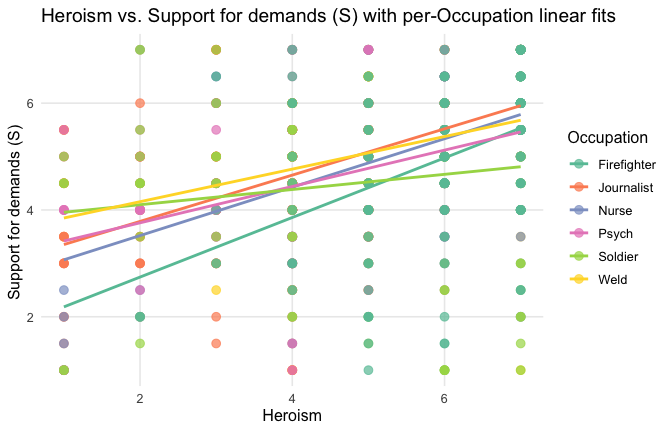

==> No support for our hypotheses. Across all occupations Heroism predicted SUPPORT for general- and specific-level workers’ demands, with or without controlling for attitude. Although effects were drastically reduced when accounting for attitude, heroism might increase our support for workers’ demands. Our hypotheses should therefore be revised.

Model 1: “~Heroism + Occupation”

# =========================
# OLD MODELS (Heroism)
# =========================
m1_H <- lm(DemandSupp_S_mean ~ Heroism + Occupation, data = scale_scores)
m2_H <- lm(DemandSupp_S_mean ~ Heroism * Occupation, data = scale_scores)
m3_H <- lm(DemandSupp_S_mean ~ Heroism + Occupation + Attitude, data = scale_scores)
m4_H <- lm(DemandSupp_S_mean ~ Heroism * Occupation + Attitude, data = scale_scores)

tidy_type3(m1_H, "~Heroism + Cond")

~Heroism + Cond
	Term	df1	df2	F	p	eta2p
Heroism	Heroism	1	833	128.46	< .001	0.134
Occupation	Occupation	5	833	3.80	= 0.002	0.022

# =========================
# NEW MODELS (Danger & Help)
# =========================

Model 2: “~Heroism * Occupation”

tidy_type3(m2_H, "~Heroism * Cond")

~Heroism * Cond
	Term	df1	df2	F	p	eta2p
Heroism	Heroism	1	828	135.61	< .001	0.141
Occupation	Occupation	5	828	2.66	= 0.021	0.016
Heroism:Occupation	Heroism:Occupation	5	828	3.63	= 0.003	0.021

Model 3: “~Heroism + Occupation + Attitude”

tidy_type3(m3_H, "~Heroism + Occupation + Attitude")

~Heroism + Occupation + Attitude
	Term	df1	df2	F	p	eta2p
Heroism	Heroism	1	832	39.50	< .001	0.045
Occupation	Occupation	5	832	3.94	= 0.002	0.023
Attitude	Attitude	1	832	6.32	= 0.012	0.008

Model 4: “~Heroism * Occupation + Attitude”

tidy_type3(m4_H, "~Heroism * Occupation + Attitude")

~Heroism * Occupation + Attitude
	Term	df1	df2	F	p	eta2p
Heroism	Heroism	1	827	39.92	< .001	0.046
Occupation	Occupation	5	827	3.42	= 0.005	0.020
Attitude	Attitude	1	827	9.75	= 0.002	0.012
Heroism:Occupation	Heroism:Occupation	5	827	4.33	< .001	0.026

Comparison of main predictors across models

# Use orthogonal contrasts; keeps your "Heroism main effect" interpretable with Cond in the model
old_contr <- options(contrasts = c("contr.sum", "contr.poly"))

# Helper to extract the main effect of "Heroism" from a car::Anova table
extract_heroism <- function(mod, model_label) {
  a <- car::Anova(mod, type = "III")

  # Coerce to data.frame with rownames preserved
  tab <- as.data.frame(a)
  tab$Term <- rownames(tab)

  # Standard column names across R versions
  # (car::Anova uses these names for lm/glm type=III)
  # Columns: "Sum Sq", "Df", "F value", "Pr(>F)"
  names(tab) <- sub(" ", "_", names(tab))  # make names safe: "Sum_Sq", "F_value", etc.

  # Pull rows we need
  hero <- tab %>% filter(Term == "Heroism")
  resid <- tab %>% filter(Term == "Residuals")

  # Safety checks (in case of name variants)
  stopifnot(nrow(hero) == 1, nrow(resid) == 1)

  # Partial eta^2 = SS_effect / (SS_effect + SS_residual)
  eta_p2 <- hero$Sum_Sq / (hero$Sum_Sq + resid$Sum_Sq)

  # Format p nicely (APA-ish)
  p_fmt <- ifelse(hero$`Pr(>F)` < .001, "< .001",
                  sprintf("= %.3f", hero$`Pr(>F)`))

  dplyr::tibble(
    Model = model_label,
    Outcome = "DemandSupp_S_mean",
    Predictor = "Heroism",
    df1 = hero$Df,
    df2 = resid$Df,
    F = hero$F_value,
    p = p_fmt,
    eta2p = eta_p2
  )
}

# ----- Fit the four models -----
mod1 <- lm(DemandSupp_S_mean ~ Heroism + Cond, data = scale_scores)
mod2 <- lm(DemandSupp_S_mean ~ Heroism * Cond, data = scale_scores)
mod3 <- lm(DemandSupp_S_mean ~ Heroism + Cond + scale(Attitude), data = scale_scores)
mod4 <- lm(DemandSupp_S_mean ~ Heroism * Cond + scale(Attitude), data = scale_scores)

# ----- Build the summary table -----
tbl <- bind_rows(
  extract_heroism(mod1, "~ Heroism + Cond"),
  extract_heroism(mod2, "~ Heroism * Occupation"),
  extract_heroism(mod3, "~ Heroism + Cond + Attitude"),
  extract_heroism(mod4, "~ Heroism * Occupation + Attitude")
  ) %>%
  # Nice number formatting for F and eta^2p
  mutate(
    F = round(F, 2),
    eta2p = round(eta2p, 3)
  )

# ----- Print as HTML-friendly table -----
# Build the table first
tbl_kbl <- tbl %>%
  kable("html",
        caption = "Main effect of Heroism across models (Type-III ANOVA): F, p, partial η²",
        align = "lllrrrcr")
# Add a footnote in a version-robust way
if ("footnote" %in% getNamespaceExports("kableExtra")) {
  tbl_kbl <- tbl_kbl %>%
    kableExtra::footnote(
      general = "Type-III sums of squares with sum contrasts. Partial η² = SS_effect / (SS_effect + SS_residual). p values are APA-style.",
      general_title = ""
    )
} else {
  tbl_kbl <- tbl_kbl %>%
    kableExtra::add_footnote(
      label = "Type-III sums of squares with sum contrasts. Partial η² = SS_effect / (SS_effect + SS_residual). p values are APA-style.",
      notation = "none"
    )
}

tbl_kbl

Main effect of Heroism across models (Type-III ANOVA): F, p, partial η²
Model	Outcome	Predictor	df1	df2	F	p	eta2p
~ Heroism + Cond	DemandSupp_S_mean	Heroism	1	833	128.46	< .001	0.134
~ Heroism * Occupation	DemandSupp_S_mean	Heroism	1	828	135.61	< .001	0.141
~ Heroism + Cond + Attitude	DemandSupp_S_mean	Heroism	1	832	39.50	< .001	0.045
~ Heroism * Occupation + Attitude	DemandSupp_S_mean	Heroism	1	827	39.92	< .001	0.046
Type-III sums of squares with sum contrasts. Partial η² = SS_effect / (SS_effect + SS_residual). p values are APA-style.

H4: Heroism is associated with decreased perception of victim-hood

The heroic status might be incompatible with the victim status (see Hartman et al., 2022) - heroes are agentic, whereas victims are passive. Heroes are there to defend us - and we might overestimate their resilience to hardship and downplay their vulnerability and suffering. At the general level, it means that we might report heroes to be less victimised, unfairly treated, exploited. At the specific level, it means we should indicate that, upon reading that 60% of the workers report intense migraines, we would feel that workers are strong enough to endure it.

General level

[How much do you see journalists as:] Victimised

Toggle details of the models diagnostics and outlier analyses

Below, you’ll find model diagnostics (QQ plot, fitted vs residuals, linearity), Outliers analysis, and more details on the output

[NOTE THAT EFFECT SIZES REPORTED IN THE REPORT COMMANDS BELOW SHOULD NOT BE TRUSTED]

paste0("####################################################")

## [1] "####################################################"

paste0("Diagnostics for Model 1: DV ~ Heroism + Occupation")

## [1] "Diagnostics for Model 1: DV ~ Heroism + Occupation"

paste0("####################################################")

## [1] "####################################################"

mod1 <- lm(Victim_G_mean ~ Heroism  + Cond, data = scale_scores)
mod1r <- lmrob(Victim_G_mean ~ Heroism  + Cond, data = scale_scores)
plot(mod1)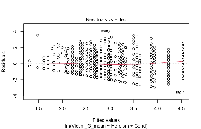

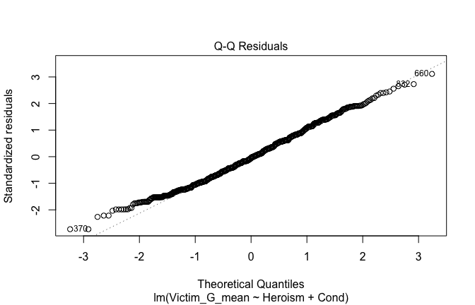
ols_plot_cooksd_bar(mod1, type = 1)

paste0("Comparison with Robust model")

## [1] "Comparison with Robust model"

models <- list("OLS (lm)" = mod1, "Robust (lmrob)" = mod1r)
modelsummary(
  models,
  statistic = c("({std.error})", "{statistic}", "p = {p.value}"),
  gof_omit  = "IC|Log.Lik",   # robust AIC comparability is iffy; omit by default
  output    = "html"
)

	OLS (lm)	Robust (lmrob)
(Intercept)	1.504	1.433
	(0.158)	(0.152)
	9.501	9.418
	p = <0.001	p = <0.001
Heroism	0.300	0.309
	(0.031)	(0.032)
	9.719	9.711
	p = <0.001	p = <0.001
Cond1	−0.623	−0.667
	(0.105)	(0.117)
	−5.952	−5.725
	p = <0.001	p = <0.001
Cond2	0.021	0.041
	(0.109)	(0.097)
	0.190	0.426
	p = 0.849	p = 0.670
Cond3	0.929	0.996
	(0.102)	(0.122)
	9.081	8.173
	p = <0.001	p = <0.001
Cond4	−0.489	−0.496
	(0.101)	(0.096)
	−4.851	−5.156
	p = <0.001	p = <0.001
Cond5	0.266	0.267
	(0.101)	(0.115)
	2.637	2.316
	p = 0.009	p = 0.021
Num.Obs.	840	840
R2	0.241	0.251
R2 Adj.	0.236	0.246
RMSE	1.29	1.30

fitted_vals <- fitted(mod1)

# Plot observed values against fitted values
plot(fitted_vals, scale_scores$Victim_G_mean,
     xlab = "Fitted Values",
     ylab = "Observed DV",
     main = "Observed vs Fitted Values")
abline(0, 1, col = "blue", lty = 2)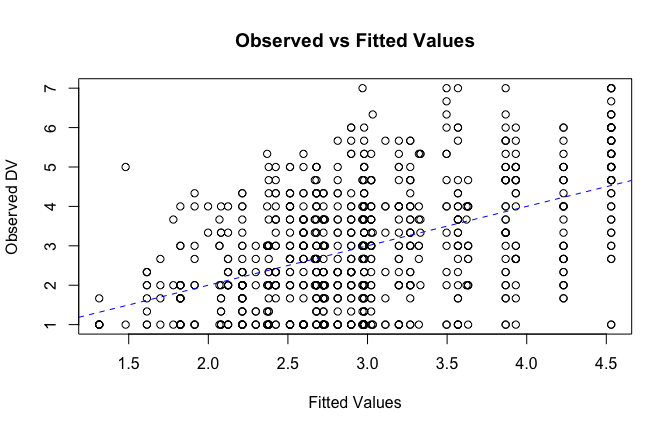

paste0("####################################################")

## [1] "####################################################"

paste0("Diagnostics for Model 2: DV ~ Heroism * Occupation")

## [1] "Diagnostics for Model 2: DV ~ Heroism * Occupation"

paste0("####################################################")

## [1] "####################################################"

mod1 <- lm(Victim_G_mean ~ Heroism  * Cond, data = scale_scores)
mod1r <- lmrob(Victim_G_mean ~ Heroism  * Cond, data = scale_scores)
plot(mod1)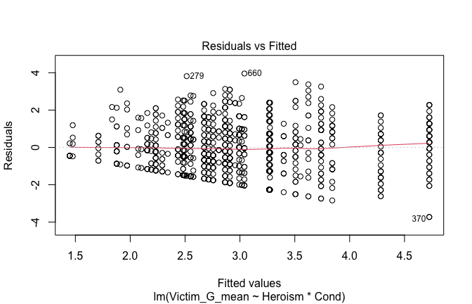

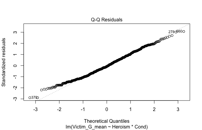
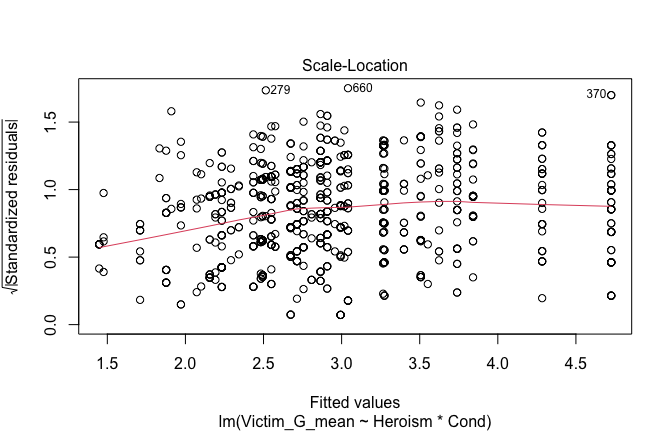
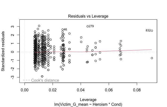
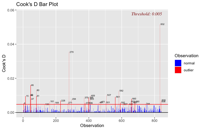
ols_plot_cooksd_bar(mod1, type = 1)

paste0("Comparison with Robust model")

## [1] "Comparison with Robust model"

models <- list("OLS (lm)" = mod1, "Robust (lmrob)" = mod1r)
modelsummary(
  models,
  statistic = c("({std.error})", "{statistic}", "p = {p.value}"),
  gof_omit  = "IC|Log.Lik",   # robust AIC comparability is iffy; omit by default
  output    = "html"
)

	OLS (lm)	Robust (lmrob)
(Intercept)	1.528	1.440
	(0.167)	(0.176)
	9.159	8.166
	p = <0.001	p = <0.001
Heroism	0.294	0.304
	(0.032)	(0.034)
	9.281	8.850
	p = <0.001	p = <0.001
Cond1	−0.000	−0.119
	(0.499)	(0.586)
	−0.001	−0.203
	p = 0.999	p = 0.840
Cond2	0.069	0.108
	(0.284)	(0.235)
	0.244	0.459
	p = 0.808	p = 0.646
Cond3	0.102	−0.069
	(0.371)	(0.411)
	0.275	−0.169
	p = 0.784	p = 0.866
Cond4	−0.342	−0.277
	(0.335)	(0.263)
	−1.020	−1.053
	p = 0.308	p = 0.292
Cond5	0.581	0.614
	(0.334)	(0.343)
	1.741	1.789
	p = 0.082	p = 0.074
Heroism × Cond1	−0.103	−0.089
	(0.084)	(0.101)
	−1.231	−0.884
	p = 0.219	p = 0.377
Heroism × Cond2	−0.015	−0.017
	(0.067)	(0.056)
	−0.222	−0.295
	p = 0.824	p = 0.768
Heroism × Cond3	0.148	0.192
	(0.065)	(0.072)
	2.279	2.682
	p = 0.023	p = 0.007
Heroism × Cond4	−0.033	−0.047
	(0.069)	(0.061)
	−0.472	−0.778
	p = 0.637	p = 0.437
Heroism × Cond5	−0.061	−0.067
	(0.063)	(0.069)
	−0.978	−0.967
	p = 0.329	p = 0.334
Num.Obs.	840	840
R2	0.248	0.261
R2 Adj.	0.238	0.251
RMSE	1.29	1.29

fitted_vals <- fitted(mod1)

# Plot observed values against fitted values
plot(fitted_vals, scale_scores$Victim_G_mean,
     xlab = "Fitted Values",
     ylab = "Observed DV",
     main = "Observed vs Fitted Values")
abline(0, 1, col = "blue", lty = 2)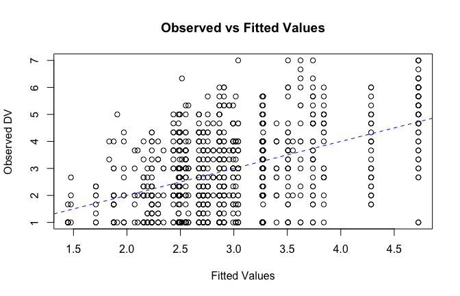

paste0("####################################################")

## [1] "####################################################"

paste0("Diagnostics for Model 3: DV ~ Heroism + Occupation + Attitude")

## [1] "Diagnostics for Model 3: DV ~ Heroism + Occupation + Attitude"

paste0("####################################################")

## [1] "####################################################"

mod1 <- lm(Victim_G_mean ~ Heroism  + Cond + Attitude, data = scale_scores)
mod1r <- lmrob(Victim_G_mean ~ Heroism  + Cond + Attitude, data = scale_scores)
plot(mod1)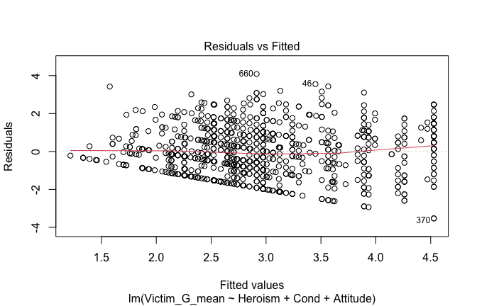

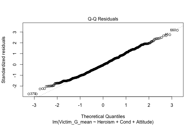
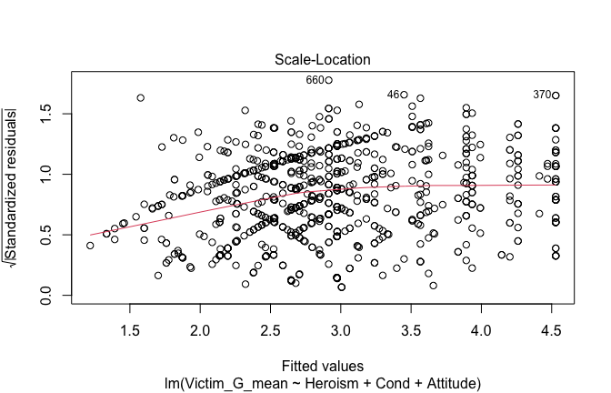
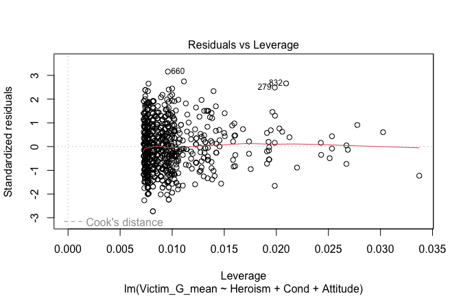
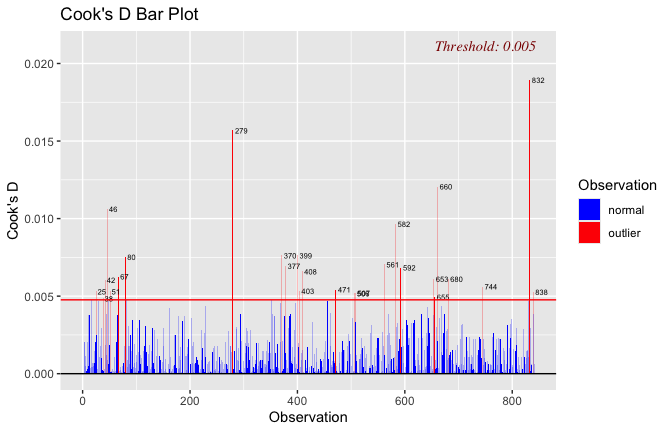
ols_plot_cooksd_bar(mod1, type = 1)

paste0("Comparison with Robust model")

## [1] "Comparison with Robust model"

models <- list("OLS (lm)" = mod1, "Robust (lmrob)" = mod1r)
modelsummary(
  models,
  statistic = c("({std.error})", "{statistic}", "p = {p.value}"),
  gof_omit  = "IC|Log.Lik",   # robust AIC comparability is iffy; omit by default
  output    = "html"
)

	OLS (lm)	Robust (lmrob)
(Intercept)	1.660	1.605
	(0.219)	(0.209)
	7.580	7.668
	p = <0.001	p = <0.001
Heroism	0.268	0.274
	(0.043)	(0.043)
	6.163	6.415
	p = <0.001	p = <0.001
Cond1	−0.638	−0.686
	(0.106)	(0.119)
	−6.038	−5.747
	p = <0.001	p = <0.001
Cond2	0.045	0.068
	(0.111)	(0.099)
	0.405	0.689
	p = 0.685	p = 0.491
Cond3	0.916	0.985
	(0.103)	(0.121)
	8.870	8.106
	p = <0.001	p = <0.001
Cond4	−0.497	−0.506
	(0.101)	(0.097)
	−4.913	−5.224
	p = <0.001	p = <0.001
Cond5	0.279	0.282
	(0.102)	(0.117)
	2.745	2.415
	p = 0.006	p = 0.016
Attitude	0.075	0.082
	(0.073)	(0.068)
	1.029	1.207
	p = 0.304	p = 0.228
Num.Obs.	840	840
R2	0.242	0.253
R2 Adj.	0.236	0.247
RMSE	1.29	1.29

fitted_vals <- fitted(mod1)

# Plot observed values against fitted values
plot(fitted_vals, scale_scores$Victim_G_mean,
     xlab = "Fitted Values",
     ylab = "Observed DV",
     main = "Observed vs Fitted Values")
abline(0, 1, col = "blue", lty = 2)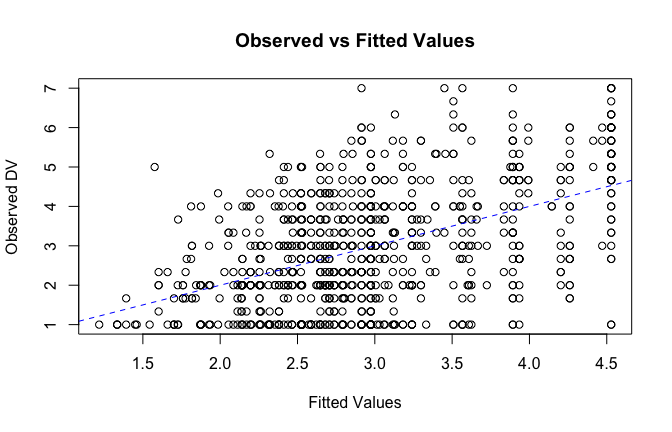

paste0("####################################################")

## [1] "####################################################"

paste0("Diagnostics for Model 4: DV ~ Heroism * Occupation + Attitude")

## [1] "Diagnostics for Model 4: DV ~ Heroism * Occupation + Attitude"

paste0("####################################################")

## [1] "####################################################"

mod1 <- lm(Victim_G_mean ~ Heroism*Cond + Attitude, data = scale_scores)
mod1r <- lmrob(Victim_G_mean ~ Heroism*Cond + Attitude, data = scale_scores)
plot(mod1)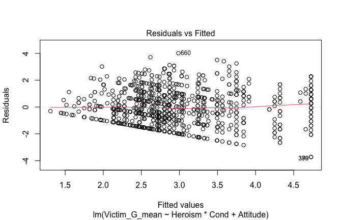

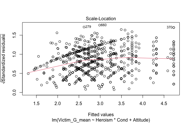
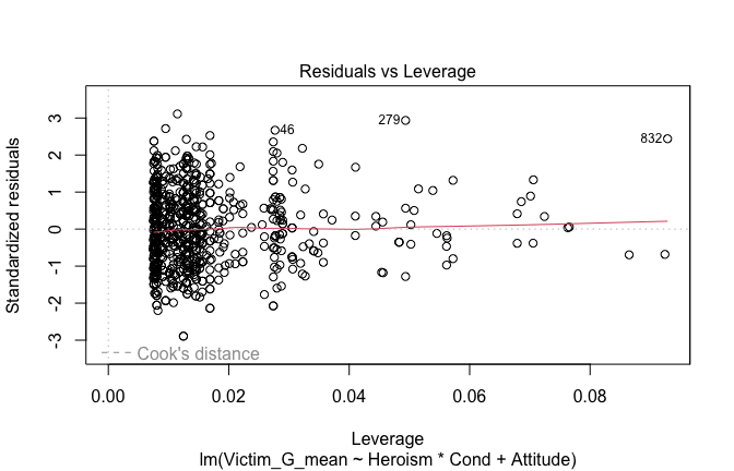
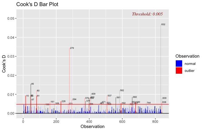
ols_plot_cooksd_bar(mod1, type = 1)

paste0("Comparison with Robust model")

## [1] "Comparison with Robust model"

models <- list("OLS (lm)" = mod1, "Robust (lmrob)" = mod1r)
modelsummary(
  models,
  statistic = c("({std.error})", "{statistic}", "p = {p.value}"),
  gof_omit  = "IC|Log.Lik",   # robust AIC comparability is iffy; omit by default
  output    = "html"
)

	OLS (lm)	Robust (lmrob)
(Intercept)	1.706	1.621
	(0.222)	(0.225)
	7.688	7.194
	p = <0.001	p = <0.001
Heroism	0.258	0.267
	(0.044)	(0.044)
	5.882	6.080
	p = <0.001	p = <0.001
Cond1	−0.072	−0.180
	(0.502)	(0.585)
	−0.142	−0.307
	p = 0.887	p = 0.759
Cond2	0.140	0.176
	(0.290)	(0.238)
	0.482	0.739
	p = 0.630	p = 0.460
Cond3	0.076	−0.076
	(0.372)	(0.405)
	0.204	−0.189
	p = 0.838	p = 0.850
Cond4	−0.371	−0.312
	(0.336)	(0.265)
	−1.105	−1.180
	p = 0.269	p = 0.238
Cond5	0.662	0.684
	(0.340)	(0.336)
	1.946	2.035
	p = 0.052	p = 0.042
Attitude	0.090	0.090
	(0.075)	(0.067)
	1.213	1.347
	p = 0.226	p = 0.178
Heroism × Cond1	−0.094	−0.083
	(0.084)	(0.101)
	−1.119	−0.818
	p = 0.263	p = 0.413
Heroism × Cond2	−0.025	−0.026
	(0.068)	(0.056)
	−0.369	−0.470
	p = 0.712	p = 0.639
Heroism × Cond3	0.150	0.192
	(0.065)	(0.071)
	2.310	2.697
	p = 0.021	p = 0.007
Heroism × Cond4	−0.027	−0.041
	(0.069)	(0.061)
	−0.394	−0.671
	p = 0.694	p = 0.502
Heroism × Cond5	−0.074	−0.077
	(0.063)	(0.068)
	−1.159	−1.135
	p = 0.247	p = 0.257
Num.Obs.	840	840
R2	0.249	0.263
R2 Adj.	0.238	0.253
RMSE	1.29	1.29

fitted_vals <- fitted(mod1)

# Plot observed values against fitted values
plot(fitted_vals, scale_scores$Victim_G_mean,
     xlab = "Fitted Values",
     ylab = "Observed DV",
     main = "Observed vs Fitted Values")
abline(0, 1, col = "blue", lty = 2)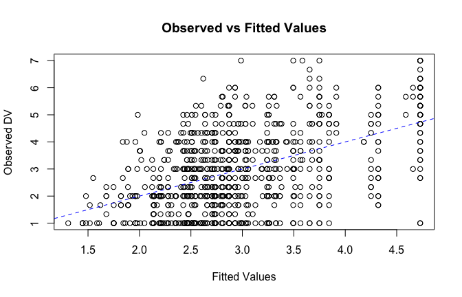

paste0("####################################################")

## [1] "####################################################"

paste0("REPORTS for each model (please ignore the eta squares, they are way off")

## [1] "REPORTS for each model (please ignore the eta squares, they are way off"

paste0("####################################################")

## [1] "####################################################"

paste0("MODEL 1: Victim_G_mean ~ Heroism")

## [1] "MODEL 1: Victim_G_mean ~ Heroism"

report(Anova(mod1 <- lm(Victim_G_mean ~ Heroism  + Cond, data = scale_scores), type = "III"))

## The ANOVA suggests that:
## 
##   - The main effect of Heroism is statistically significant and medium (F(1, 833)
## = 94.47, p < .001; Eta2 (partial) = 0.10, 95% CI [0.07, 1.00])
##   - The main effect of Cond is statistically significant and medium (F(5, 833) =
## 26.21, p < .001; Eta2 (partial) = 0.14, 95% CI [0.10, 1.00])
## 
## Effect sizes were labelled following Field's (2013) recommendations.

paste0("MODEL 2: Victim_G_mean ~ Heroism * Cond")

## [1] "MODEL 2: Victim_G_mean ~ Heroism * Cond"

report(Anova(mod2 <- lm(Victim_G_mean ~ Heroism * Cond, data = scale_scores), type = "III"))

## Type 3 ANOVAs only give sensible and informative results when covariates
##   are mean-centered and factors are coded with orthogonal contrasts (such
##   as those produced by `contr.sum`, `contr.poly`, or `contr.helmert`, but
##   *not* by the default `contr.treatment`).

## The ANOVA suggests that:
## 
##   - The main effect of Heroism is statistically significant and medium (F(1, 828)
## = 86.13, p < .001; Eta2 (partial) = 0.09, 95% CI [0.07, 1.00])
##   - The main effect of Cond is statistically not significant and very small (F(5,
## 828) = 0.94, p = 0.457; Eta2 (partial) = 5.61e-03, 95% CI [0.00, 1.00])
##   - The interaction between Heroism and Cond is statistically not significant and
## very small (F(5, 828) = 1.47, p = 0.197; Eta2 (partial) = 8.81e-03, 95% CI
## [0.00, 1.00])
## 
## Effect sizes were labelled following Field's (2013) recommendations.

paste0("MODEL 3: Victim_G_mean ~ Heroism +scale(Attitude)")

## [1] "MODEL 3: Victim_G_mean ~ Heroism +scale(Attitude)"

report(Anova(mod3 <- lm(Victim_G_mean ~ Heroism   + Cond +scale(Attitude) , data = scale_scores), type = "III"))

## The ANOVA suggests that:
## 
##   - The main effect of Heroism is statistically significant and small (F(1, 832)
## = 37.98, p < .001; Eta2 (partial) = 0.04, 95% CI [0.02, 1.00])
##   - The main effect of Cond is statistically significant and medium (F(5, 832) =
## 26.36, p < .001; Eta2 (partial) = 0.14, 95% CI [0.10, 1.00])
##   - The main effect of scale(Attitude) is statistically not significant and very
## small (F(1, 832) = 1.06, p = 0.304; Eta2 (partial) = 1.27e-03, 95% CI [0.00,
## 1.00])
## 
## Effect sizes were labelled following Field's (2013) recommendations.

paste0("MODEL 4: Victim_G_mean ~ Heroism * Cond + scale(Attitude)")

## [1] "MODEL 4: Victim_G_mean ~ Heroism * Cond + scale(Attitude)"

report(Anova(mod4 <-lm(Victim_G_mean ~ Heroism * Cond + scale(Attitude), data = scale_scores), type = "III"))

## Type 3 ANOVAs only give sensible and informative results when covariates
##   are mean-centered and factors are coded with orthogonal contrasts (such
##   as those produced by `contr.sum`, `contr.poly`, or `contr.helmert`, but
##   *not* by the default `contr.treatment`).

## The ANOVA suggests that:
## 
##   - The main effect of Heroism is statistically significant and small (F(1, 827)
## = 34.60, p < .001; Eta2 (partial) = 0.04, 95% CI [0.02, 1.00])
##   - The main effect of Cond is statistically not significant and very small (F(5,
## 827) = 1.12, p = 0.347; Eta2 (partial) = 6.74e-03, 95% CI [0.00, 1.00])
##   - The main effect of scale(Attitude) is statistically not significant and very
## small (F(1, 827) = 1.47, p = 0.226; Eta2 (partial) = 1.78e-03, 95% CI [0.00,
## 1.00])
##   - The interaction between Heroism and Cond is statistically not significant and
## very small (F(5, 827) = 1.55, p = 0.171; Eta2 (partial) = 9.31e-03, 95% CI
## [0.00, 1.00])
## 
## Effect sizes were labelled following Field's (2013) recommendations.

paste0("Model Comparison: assessing the importance of attitude - not accounting for occupations")

## [1] "Model Comparison: assessing the importance of attitude - not accounting for occupations"

anova(mod1, mod3)

paste0("Model Comparison: assessing the importance of attitude - accounting for occupations")

## [1] "Model Comparison: assessing the importance of attitude - accounting for occupations"

anova(mod2, mod4)

ggplot(scale_scores, aes(y = Victim_G_mean, x = Heroism)) +
  # 1) points colored by Cond
  geom_point(aes(color = Cond),
             size = 2.7, alpha = 0.7) +
  
  # 2) ONE global lm line (group = 1 prevents one line per Cond)
  stat_smooth(method = "lm", se = TRUE,
              aes(group = 1),
              color = "black", linewidth = 1) +
  
  # Nice, accessible palette (works well with >3 groups)
  scale_color_brewer(palette = "Set2") +
  
  labs(
    y = "Victimisation (G)",
    x = "Heroism",
    color = "Occupation",
    title = "Heroism vs. Victimisation (G), colored by Occupation",
    subtitle = "Points are participants; black line is overall linear fit with 95% CI"
  ) +
  theme_minimal(base_size = 12) +
  theme(
    legend.position = "right",
    panel.grid.minor = element_blank()
  )

## `geom_smooth()` using formula = 'y ~ x'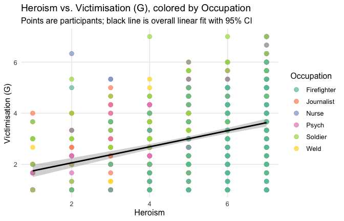

ggplot(scale_scores, aes(y = Victim_G_mean, x = Heroism, color = Cond)) +
  # points colored by condition
  geom_point(size = 2.7, alpha = 0.7) +
  # ONE lm line PER condition (because color is mapped here)
  stat_smooth(method = "lm", se = FALSE, linewidth = 1, fullrange = TRUE) +
  scale_color_brewer(palette = "Set2") +
  labs(
    y = "Victimisation (G)",
    x = "Heroism",
    color = "Occupation",
    title = "Heroism vs. Victimisation (G) with per-Occupation linear fits"
  ) +
  theme_minimal(base_size = 12) +
  theme(legend.position = "right", panel.grid.minor = element_blank())

## `geom_smooth()` using formula = 'y ~ x'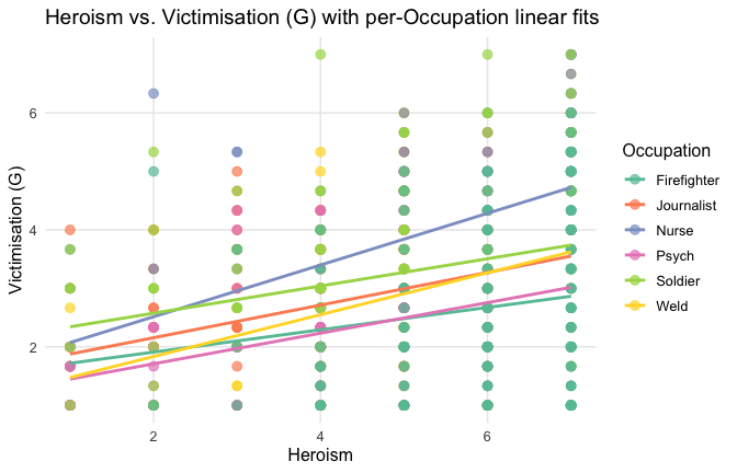

A significant, yet small effect, in the opposite direction.

Model 1: “~Heroism + Occupation”

# =========================
# OLD MODELS (Heroism)
# =========================
m1_H <- lm(Victim_G_mean ~ Heroism + Occupation, data = scale_scores)
m2_H <- lm(Victim_G_mean ~ Heroism * Occupation, data = scale_scores)
m3_H <- lm(Victim_G_mean ~ Heroism + Occupation + Attitude, data = scale_scores)
m4_H <- lm(Victim_G_mean ~ Heroism * Occupation + Attitude, data = scale_scores)

tidy_type3(m1_H, "~Heroism + Cond")

~Heroism + Cond
	Term	df1	df2	F	p	eta2p
Heroism	Heroism	1	833	94.47	< .001	0.102
Occupation	Occupation	5	833	26.21	< .001	0.136

# =========================
# NEW MODELS (Danger & Help)
# =========================

Model 2: “~Heroism * Occupation”

tidy_type3(m2_H, "~Heroism * Cond")

~Heroism * Cond
	Term	df1	df2	F	p	eta2p
Heroism	Heroism	1	828	86.13	< .001	0.094
Occupation	Occupation	5	828	0.94	= 0.457	0.006
Heroism:Occupation	Heroism:Occupation	5	828	1.47	= 0.197	0.009

Model 3: “~Heroism + Occupation + Attitude”

tidy_type3(m3_H, "~Heroism + Occupation + Attitude")

~Heroism + Occupation + Attitude
	Term	df1	df2	F	p	eta2p
Heroism	Heroism	1	832	37.98	< .001	0.044
Occupation	Occupation	5	832	26.36	< .001	0.137
Attitude	Attitude	1	832	1.06	= 0.304	0.001

Model 4: “~Heroism * Occupation + Attitude”

tidy_type3(m4_H, "~Heroism * Occupation + Attitude")

~Heroism * Occupation + Attitude
	Term	df1	df2	F	p	eta2p
Heroism	Heroism	1	827	34.60	< .001	0.040
Occupation	Occupation	5	827	1.12	= 0.347	0.007
Attitude	Attitude	1	827	1.47	= 0.226	0.002
Heroism:Occupation	Heroism:Occupation	5	827	1.55	= 0.171	0.009

Comparison of main predictors across models

# Use orthogonal contrasts; keeps your "Heroism main effect" interpretable with Cond in the model
old_contr <- options(contrasts = c("contr.sum", "contr.poly"))

# Helper to extract the main effect of "Heroism" from a car::Anova table
extract_heroism <- function(mod, model_label) {
  a <- car::Anova(mod, type = "III")

  # Coerce to data.frame with rownames preserved
  tab <- as.data.frame(a)
  tab$Term <- rownames(tab)

  # Standard column names across R versions
  # (car::Anova uses these names for lm/glm type=III)
  # Columns: "Sum Sq", "Df", "F value", "Pr(>F)"
  names(tab) <- sub(" ", "_", names(tab))  # make names safe: "Sum_Sq", "F_value", etc.

  # Pull rows we need
  hero <- tab %>% filter(Term == "Heroism")
  resid <- tab %>% filter(Term == "Residuals")

  # Safety checks (in case of name variants)
  stopifnot(nrow(hero) == 1, nrow(resid) == 1)

  # Partial eta^2 = SS_effect / (SS_effect + SS_residual)
  eta_p2 <- hero$Sum_Sq / (hero$Sum_Sq + resid$Sum_Sq)

  # Format p nicely (APA-ish)
  p_fmt <- ifelse(hero$`Pr(>F)` < .001, "< .001",
                  sprintf("= %.3f", hero$`Pr(>F)`))

  dplyr::tibble(
    Model = model_label,
    Outcome = "Victim_G_mean",
    Predictor = "Heroism",
    df1 = hero$Df,
    df2 = resid$Df,
    F = hero$F_value,
    p = p_fmt,
    eta2p = eta_p2
  )
}

# ----- Fit the four models -----
mod1 <- lm(Victim_G_mean ~ Heroism + Cond, data = scale_scores)
mod2 <- lm(Victim_G_mean ~ Heroism * Cond, data = scale_scores)
mod3 <- lm(Victim_G_mean ~ Heroism + Cond + scale(Attitude), data = scale_scores)
mod4 <- lm(Victim_G_mean ~ Heroism * Cond + scale(Attitude), data = scale_scores)

# ----- Build the summary table -----
tbl <- bind_rows(
  extract_heroism(mod1, "~ Heroism + Occupation"),
  extract_heroism(mod2, "~ Heroism * Occupation"),
  extract_heroism(mod3, "~ Heroism + Occupation + Attitude"),
  extract_heroism(mod4, "~ Heroism * Occupation + Attitude")
  ) %>%
  # Nice number formatting for F and eta^2p
  mutate(
    F = round(F, 2),
    eta2p = round(eta2p, 3)
  )

# ----- Print as HTML-friendly table -----
# Build the table first
tbl_kbl <- tbl %>%
  kable("html",
        caption = "Main effect of Heroism across models (Type-III ANOVA): F, p, partial η²",
        align = "lllrrrcr")
# Add a footnote in a version-robust way
if ("footnote" %in% getNamespaceExports("kableExtra")) {
  tbl_kbl <- tbl_kbl %>%
    kableExtra::footnote(
      general = "Type-III sums of squares with sum contrasts. Partial η² = SS_effect / (SS_effect + SS_residual). p values are APA-style.",
      general_title = ""
    )
} else {
  tbl_kbl <- tbl_kbl %>%
    kableExtra::add_footnote(
      label = "Type-III sums of squares with sum contrasts. Partial η² = SS_effect / (SS_effect + SS_residual). p values are APA-style.",
      notation = "none"
    )
}

tbl_kbl

Main effect of Heroism across models (Type-III ANOVA): F, p, partial η²
Model	Outcome	Predictor	df1	df2	F	p	eta2p
~ Heroism + Occupation	Victim_G_mean	Heroism	1	833	94.47	< .001	0.102
~ Heroism * Occupation	Victim_G_mean	Heroism	1	828	86.13	< .001	0.094
~ Heroism + Occupation + Attitude	Victim_G_mean	Heroism	1	832	37.98	< .001	0.044
~ Heroism * Occupation + Attitude	Victim_G_mean	Heroism	1	827	34.60	< .001	0.040
Type-III sums of squares with sum contrasts. Partial η² = SS_effect / (SS_effect + SS_residual). p values are APA-style.

Specific level

[Consider the following observation from a recent report: In their professional life, more than 60% of journalists have reported intense migraines from working long hours. How much would you agree or disagree with the following statements:] I believe journalists are strong enough to face this condition

Toggle details of the models diagnostics and outlier analyses

Below, you’ll find model diagnostics (QQ plot, fitted vs residuals, linearity), Outliers analysis, and more details on the output

[NOTE THAT EFFECT SIZES REPORTED IN THE REPORT COMMANDS BELOW SHOULD NOT BE TRUSTED]

paste0("####################################################")

## [1] "####################################################"

paste0("Diagnostics for Model 1: DV ~ Heroism + Occupation")

## [1] "Diagnostics for Model 1: DV ~ Heroism + Occupation"

paste0("####################################################")

## [1] "####################################################"

mod1 <- lm(Victim_S_mean ~ Heroism  + Cond, data = scale_scores)
mod1r <- lmrob(Victim_S_mean ~ Heroism  + Cond, data = scale_scores)
plot(mod1)

ols_plot_cooksd_bar(mod1, type = 1)

paste0("Comparison with Robust model")

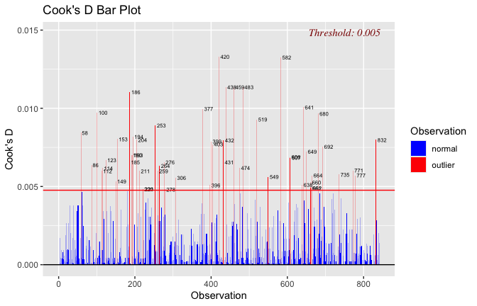
## [1] "Comparison with Robust model"

models <- list("OLS (lm)" = mod1, "Robust (lmrob)" = mod1r)
modelsummary(
  models,
  statistic = c("({std.error})", "{statistic}", "p = {p.value}"),
  gof_omit  = "IC|Log.Lik",   # robust AIC comparability is iffy; omit by default
  output    = "html"
)

	OLS (lm)	Robust (lmrob)
(Intercept)	3.376	3.322
	(0.132)	(0.162)
	25.614	20.518
	p = <0.001	p = <0.001
Heroism	0.291	0.309
	(0.026)	(0.030)
	11.342	10.185
	p = <0.001	p = <0.001
Cond1	0.040	0.016
	(0.087)	(0.081)
	0.462	0.194
	p = 0.644	p = 0.846
Cond2	−0.559	−0.515
	(0.091)	(0.107)
	−6.167	−4.820
	p = <0.001	p = <0.001
Cond3	0.380	0.361
	(0.085)	(0.079)
	4.462	4.572
	p = <0.001	p = <0.001
Cond4	−0.126	−0.115
	(0.084)	(0.080)
	−1.499	−1.432
	p = 0.134	p = 0.153
Cond5	−0.192	−0.230
	(0.084)	(0.098)
	−2.287	−2.357
	p = 0.022	p = 0.019
Num.Obs.	840	840
R2	0.280	0.300
R2 Adj.	0.275	0.295
RMSE	1.08	1.08

fitted_vals <- fitted(mod1)

# Plot observed values against fitted values
plot(fitted_vals, scale_scores$Victim_S_mean,
     xlab = "Fitted Values",
     ylab = "Observed DV",
     main = "Observed vs Fitted Values")
abline(0, 1, col = "blue", lty = 2)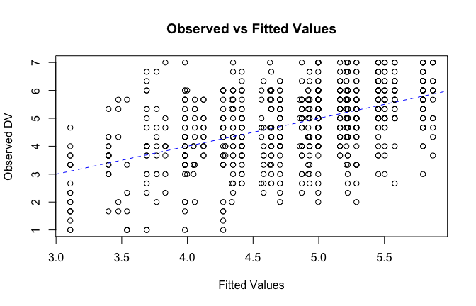

paste0("####################################################")

## [1] "####################################################"

paste0("Diagnostics for Model 2: DV ~ Heroism * Occupation")

## [1] "Diagnostics for Model 2: DV ~ Heroism * Occupation"

paste0("####################################################")

## [1] "####################################################"

mod1 <- lm(Victim_S_mean ~ Heroism  * Cond, data = scale_scores)
mod1r <- lmrob(Victim_S_mean ~ Heroism  * Cond, data = scale_scores)
plot(mod1)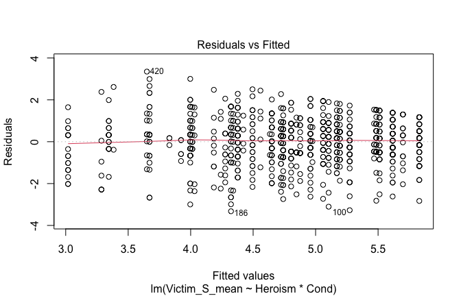

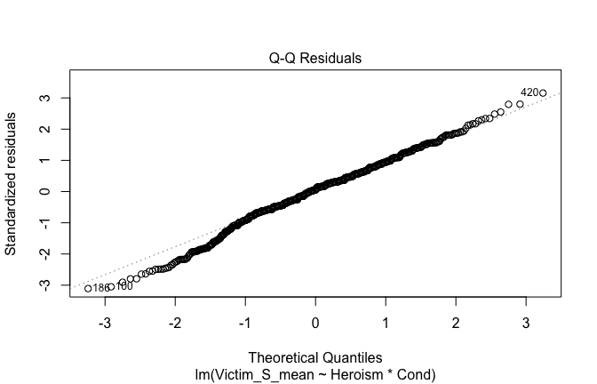
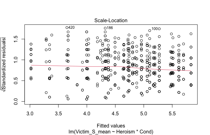
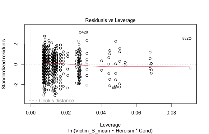
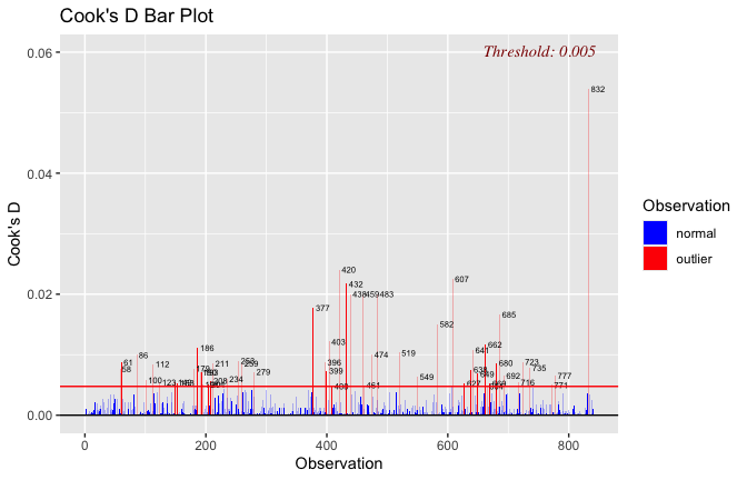
ols_plot_cooksd_bar(mod1, type = 1)

paste0("Comparison with Robust model")

## [1] "Comparison with Robust model"

models <- list("OLS (lm)" = mod1, "Robust (lmrob)" = mod1r)
modelsummary(
  models,
  statistic = c("({std.error})", "{statistic}", "p = {p.value}"),
  gof_omit  = "IC|Log.Lik",   # robust AIC comparability is iffy; omit by default
  output    = "html"
)

	OLS (lm)	Robust (lmrob)
(Intercept)	3.299	3.249
	(0.138)	(0.158)
	23.834	20.595
	p = <0.001	p = <0.001
Heroism	0.304	0.321
	(0.026)	(0.029)
	11.546	11.038
	p = <0.001	p = <0.001
Cond1	−0.809	−0.964
	(0.414)	(0.426)
	−1.955	−2.261
	p = 0.051	p = 0.024
Cond2	−0.606	−0.623
	(0.235)	(0.257)
	−2.577	−2.427
	p = 0.010	p = 0.015
Cond3	0.306	0.323
	(0.308)	(0.328)
	0.993	0.985
	p = 0.321	p = 0.325
Cond4	−0.377	−0.410
	(0.278)	(0.379)
	−1.357	−1.082
	p = 0.175	p = 0.280
Cond5	0.577	0.702
	(0.277)	(0.402)
	2.085	1.745
	p = 0.037	p = 0.081
Heroism × Cond1	0.143	0.162
	(0.070)	(0.070)
	2.058	2.329
	p = 0.040	p = 0.020
Heroism × Cond2	0.022	0.039
	(0.056)	(0.060)
	0.401	0.658
	p = 0.688	p = 0.511
Heroism × Cond3	0.014	0.007
	(0.054)	(0.055)
	0.264	0.128
	p = 0.792	p = 0.898
Heroism × Cond4	0.060	0.066
	(0.057)	(0.074)
	1.050	0.892
	p = 0.294	p = 0.373
Heroism × Cond5	−0.149	−0.177
	(0.052)	(0.072)
	−2.866	−2.463
	p = 0.004	p = 0.014
Num.Obs.	840	840
R2	0.292	0.314
R2 Adj.	0.282	0.305
RMSE	1.07	1.07

fitted_vals <- fitted(mod1)

# Plot observed values against fitted values
plot(fitted_vals, scale_scores$Victim_S_mean,
     xlab = "Fitted Values",
     ylab = "Observed DV",
     main = "Observed vs Fitted Values")
abline(0, 1, col = "blue", lty = 2)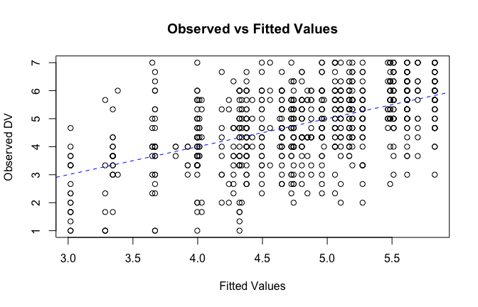

paste0("####################################################")

## [1] "####################################################"

paste0("Diagnostics for Model 3: DV ~ Heroism + Occupation + Attitude")

## [1] "Diagnostics for Model 3: DV ~ Heroism + Occupation + Attitude"

paste0("####################################################")

## [1] "####################################################"

mod1 <- lm(Victim_S_mean ~ Heroism  + Cond + Attitude, data = scale_scores)
mod1r <- lmrob(Victim_S_mean ~ Heroism  + Cond + Attitude, data = scale_scores)
plot(mod1)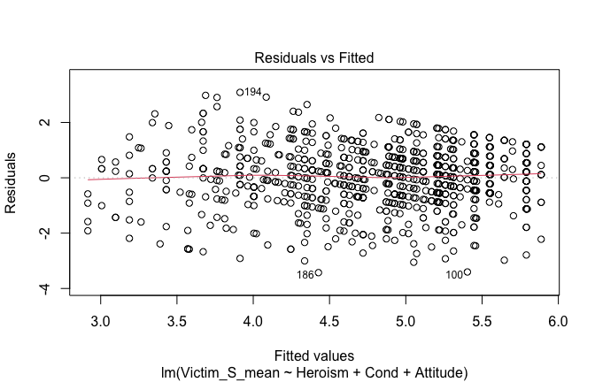

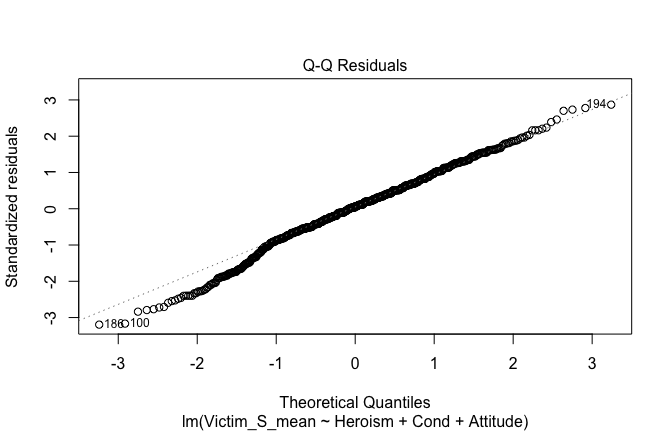
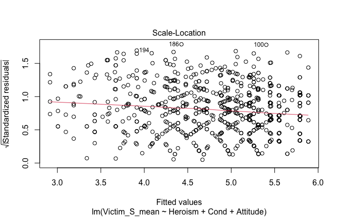
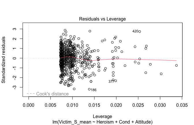
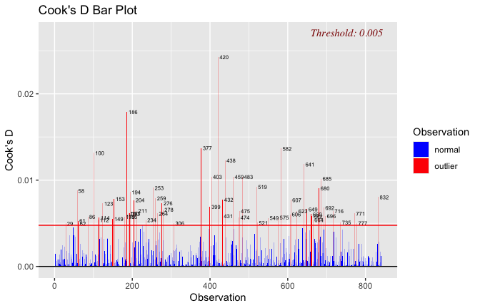
ols_plot_cooksd_bar(mod1, type = 1)

paste0("Comparison with Robust model")

## [1] "Comparison with Robust model"

models <- list("OLS (lm)" = mod1, "Robust (lmrob)" = mod1r)
modelsummary(
  models,
  statistic = c("({std.error})", "{statistic}", "p = {p.value}"),
  gof_omit  = "IC|Log.Lik",   # robust AIC comparability is iffy; omit by default
  output    = "html"
)

	OLS (lm)	Robust (lmrob)
(Intercept)	3.619	3.659
	(0.182)	(0.217)
	19.883	16.894
	p = <0.001	p = <0.001
Heroism	0.242	0.241
	(0.036)	(0.042)
	6.688	5.771
	p = <0.001	p = <0.001
Cond1	0.015	−0.020
	(0.088)	(0.081)
	0.176	−0.248
	p = 0.860	p = 0.804
Cond2	−0.520	−0.459
	(0.093)	(0.110)
	−5.624	−4.162
	p = <0.001	p = <0.001
Cond3	0.359	0.329
	(0.086)	(0.078)
	4.180	4.234
	p = <0.001	p = <0.001
Cond4	−0.138	−0.125
	(0.084)	(0.080)
	−1.638	−1.568
	p = 0.102	p = 0.117
Cond5	−0.172	−0.212
	(0.085)	(0.100)
	−2.032	−2.108
	p = 0.043	p = 0.035
Attitude	0.117	0.164
	(0.061)	(0.072)
	1.933	2.274
	p = 0.054	p = 0.023
Num.Obs.	840	840
R2	0.284	0.309
R2 Adj.	0.278	0.304
RMSE	1.08	1.08

fitted_vals <- fitted(mod1)

# Plot observed values against fitted values
plot(fitted_vals, scale_scores$Victim_S_mean,
     xlab = "Fitted Values",
     ylab = "Observed DV",
     main = "Observed vs Fitted Values")
abline(0, 1, col = "blue", lty = 2)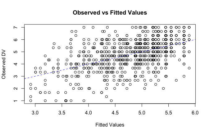

paste0("####################################################")

## [1] "####################################################"

paste0("Diagnostics for Model 4: DV ~ Heroism * Occupation + Attitude")

## [1] "Diagnostics for Model 4: DV ~ Heroism * Occupation + Attitude"

paste0("####################################################")

## [1] "####################################################"

mod1 <- lm(Victim_S_mean ~ Heroism*Cond + Attitude, data = scale_scores)
mod1r <- lmrob(Victim_S_mean ~ Heroism*Cond + Attitude, data = scale_scores)
plot(mod1)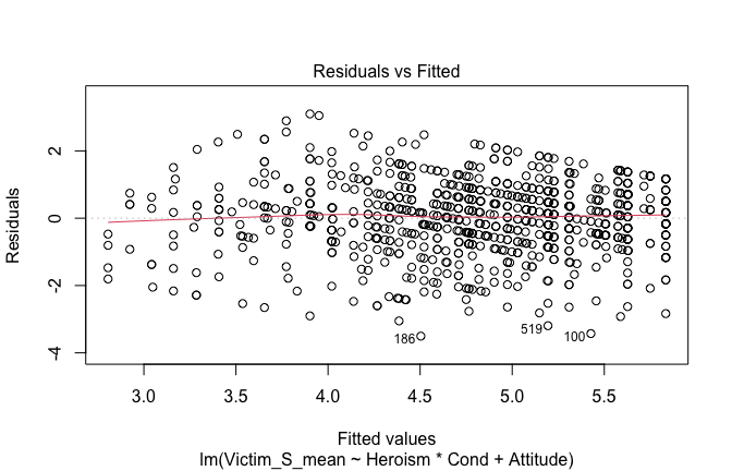

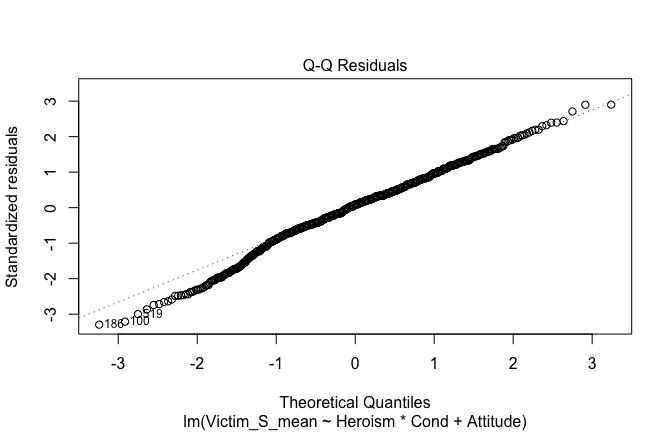
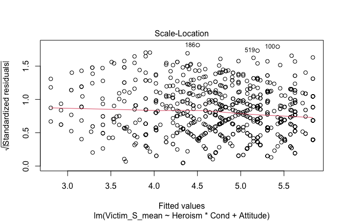
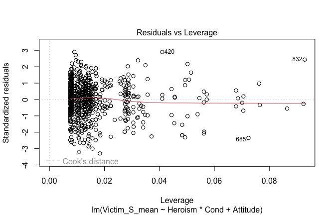
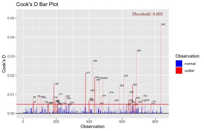
ols_plot_cooksd_bar(mod1, type = 1)

paste0("Comparison with Robust model")

## [1] "Comparison with Robust model"

models <- list("OLS (lm)" = mod1, "Robust (lmrob)" = mod1r)
modelsummary(
  models,
  statistic = c("({std.error})", "{statistic}", "p = {p.value}"),
  gof_omit  = "IC|Log.Lik",   # robust AIC comparability is iffy; omit by default
  output    = "html"
)

	OLS (lm)	Robust (lmrob)
(Intercept)	3.599	3.655
	(0.184)	(0.225)
	19.611	16.249
	p = <0.001	p = <0.001
Heroism	0.242	0.239
	(0.036)	(0.043)
	6.674	5.585
	p = <0.001	p = <0.001
Cond1	−0.929	−1.108
	(0.415)	(0.418)
	−2.237	−2.649
	p = 0.026	p = 0.008
Cond2	−0.487	−0.506
	(0.239)	(0.252)
	−2.035	−2.010
	p = 0.042	p = 0.045
Cond3	0.262	0.294
	(0.308)	(0.302)
	0.852	0.974
	p = 0.395	p = 0.330
Cond4	−0.426	−0.463
	(0.278)	(0.375)
	−1.536	−1.235
	p = 0.125	p = 0.217
Cond5	0.715	0.892
	(0.282)	(0.431)
	2.538	2.069
	p = 0.011	p = 0.039
Attitude	0.153	0.197
	(0.062)	(0.071)
	2.476	2.778
	p = 0.013	p = 0.006
Heroism × Cond1	0.158	0.180
	(0.070)	(0.068)
	2.276	2.631
	p = 0.023	p = 0.009
Heroism × Cond2	0.005	0.026
	(0.056)	(0.059)
	0.095	0.435
	p = 0.924	p = 0.664
Heroism × Cond3	0.018	0.006
	(0.054)	(0.051)
	0.329	0.118
	p = 0.742	p = 0.906
Heroism × Cond4	0.069	0.076
	(0.057)	(0.074)
	1.209	1.029
	p = 0.227	p = 0.304
Heroism × Cond5	−0.170	−0.206
	(0.053)	(0.076)
	−3.233	−2.727
	p = 0.001	p = 0.007
Num.Obs.	840	840
R2	0.297	0.324
R2 Adj.	0.287	0.314
RMSE	1.07	1.07

fitted_vals <- fitted(mod1)

# Plot observed values against fitted values
plot(fitted_vals, scale_scores$Victim_S_mean,
     xlab = "Fitted Values",
     ylab = "Observed DV",
     main = "Observed vs Fitted Values")
abline(0, 1, col = "blue", lty = 2)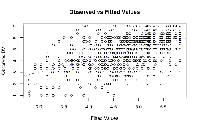

paste0("####################################################")

## [1] "####################################################"

paste0("REPORTS for each model (please ignore the eta squares, they are way off")

## [1] "REPORTS for each model (please ignore the eta squares, they are way off"

paste0("####################################################")

## [1] "####################################################"

paste0("MODEL 1: Victim_S_mean ~ Heroism")

## [1] "MODEL 1: Victim_S_mean ~ Heroism"

report(Anova(mod1 <- lm(Victim_S_mean ~ Heroism  + Cond, data = scale_scores), type = "III"))

## The ANOVA suggests that:
## 
##   - The main effect of Heroism is statistically significant and medium (F(1, 833)
## = 128.64, p < .001; Eta2 (partial) = 0.13, 95% CI [0.10, 1.00])
##   - The main effect of Cond is statistically significant and medium (F(5, 833) =
## 15.52, p < .001; Eta2 (partial) = 0.09, 95% CI [0.05, 1.00])
## 
## Effect sizes were labelled following Field's (2013) recommendations.

paste0("MODEL 2: Victim_S_mean ~ Heroism * Cond")

## [1] "MODEL 2: Victim_S_mean ~ Heroism * Cond"

report(Anova(mod2 <- lm(Victim_S_mean ~ Heroism * Cond, data = scale_scores), type = "III"))

## Type 3 ANOVAs only give sensible and informative results when covariates
##   are mean-centered and factors are coded with orthogonal contrasts (such
##   as those produced by `contr.sum`, `contr.poly`, or `contr.helmert`, but
##   *not* by the default `contr.treatment`).

## The ANOVA suggests that:
## 
##   - The main effect of Heroism is statistically significant and medium (F(1, 828)
## = 133.32, p < .001; Eta2 (partial) = 0.14, 95% CI [0.10, 1.00])
##   - The main effect of Cond is statistically significant and small (F(5, 828) =
## 4.55, p < .001; Eta2 (partial) = 0.03, 95% CI [7.74e-03, 1.00])
##   - The interaction between Heroism and Cond is statistically significant and
## small (F(5, 828) = 2.65, p = 0.022; Eta2 (partial) = 0.02, 95% CI [1.21e-03,
## 1.00])
## 
## Effect sizes were labelled following Field's (2013) recommendations.

paste0("MODEL 3: Victim_S_mean ~ Heroism +scale(Attitude)")

## [1] "MODEL 3: Victim_S_mean ~ Heroism +scale(Attitude)"

report(Anova(mod3 <- lm(Victim_S_mean ~ Heroism   + Cond +scale(Attitude) , data = scale_scores), type = "III"))

## The ANOVA suggests that:
## 
##   - The main effect of Heroism is statistically significant and small (F(1, 832)
## = 44.73, p < .001; Eta2 (partial) = 0.05, 95% CI [0.03, 1.00])
##   - The main effect of Cond is statistically significant and medium (F(5, 832) =
## 13.87, p < .001; Eta2 (partial) = 0.08, 95% CI [0.05, 1.00])
##   - The main effect of scale(Attitude) is statistically not significant and very
## small (F(1, 832) = 3.74, p = 0.054; Eta2 (partial) = 4.47e-03, 95% CI [0.00,
## 1.00])
## 
## Effect sizes were labelled following Field's (2013) recommendations.

paste0("MODEL 4: Victim_S_mean ~ Heroism * Cond + scale(Attitude)")

## [1] "MODEL 4: Victim_S_mean ~ Heroism * Cond + scale(Attitude)"

report(Anova(mod4 <-lm(Victim_S_mean ~ Heroism * Cond + scale(Attitude), data = scale_scores), type = "III"))

## Type 3 ANOVAs only give sensible and informative results when covariates
##   are mean-centered and factors are coded with orthogonal contrasts (such
##   as those produced by `contr.sum`, `contr.poly`, or `contr.helmert`, but
##   *not* by the default `contr.treatment`).

## The ANOVA suggests that:
## 
##   - The main effect of Heroism is statistically significant and small (F(1, 827)
## = 44.54, p < .001; Eta2 (partial) = 0.05, 95% CI [0.03, 1.00])
##   - The main effect of Cond is statistically significant and small (F(5, 827) =
## 4.62, p < .001; Eta2 (partial) = 0.03, 95% CI [8.02e-03, 1.00])
##   - The main effect of scale(Attitude) is statistically significant and very
## small (F(1, 827) = 6.13, p = 0.013; Eta2 (partial) = 7.36e-03, 95% CI
## [8.18e-04, 1.00])
##   - The interaction between Heroism and Cond is statistically significant and
## small (F(5, 827) = 3.14, p = 0.008; Eta2 (partial) = 0.02, 95% CI [2.74e-03,
## 1.00])
## 
## Effect sizes were labelled following Field's (2013) recommendations.

paste0("Model Comparison: assessing the importance of attitude - not accounting for occupations")

## [1] "Model Comparison: assessing the importance of attitude - not accounting for occupations"

anova(mod1, mod3)

paste0("Model Comparison: assessing the importance of attitude - accounting for occupations")

## [1] "Model Comparison: assessing the importance of attitude - accounting for occupations"

anova(mod2, mod4)

ggplot(scale_scores, aes(y = Victim_S_mean, x = Heroism)) +
  # 1) points colored by Cond
  geom_point(aes(color = Cond),
             size = 2.7, alpha = 0.7) +
  
  # 2) ONE global lm line (group = 1 prevents one line per Cond)
  stat_smooth(method = "lm", se = TRUE,
              aes(group = 1),
              color = "black", linewidth = 1) +
  
  # Nice, accessible palette (works well with >3 groups)
  scale_color_brewer(palette = "Set2") +
  
  labs(
    y = "Victimisation (S)",
    x = "Heroism",
    color = "Occupation",
    title = "Heroism vs. Victimisation (S), colored by Occupation",
    subtitle = "Points are participants; black line is overall linear fit with 95% CI"
  ) +
  theme_minimal(base_size = 12) +
  theme(
    legend.position = "right",
    panel.grid.minor = element_blank()
  )

## `geom_smooth()` using formula = 'y ~ x'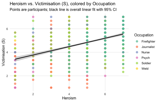

ggplot(scale_scores, aes(y = Victim_S_mean, x = Heroism, color = Cond)) +
  # points colored by condition
  geom_point(size = 2.7, alpha = 0.7) +
  # ONE lm line PER condition (because color is mapped here)
  stat_smooth(method = "lm", se = FALSE, linewidth = 1, fullrange = TRUE) +
  scale_color_brewer(palette = "Set2") +
  labs(
    y = "Victimisation (S)",
    x = "Heroism",
    color = "Occupation",
    title = "Heroism vs. Victimisation (S) with per-Occupation linear fits"
  ) +
  theme_minimal(base_size = 12) +
  theme(legend.position = "right", panel.grid.minor = element_blank())

## `geom_smooth()` using formula = 'y ~ x'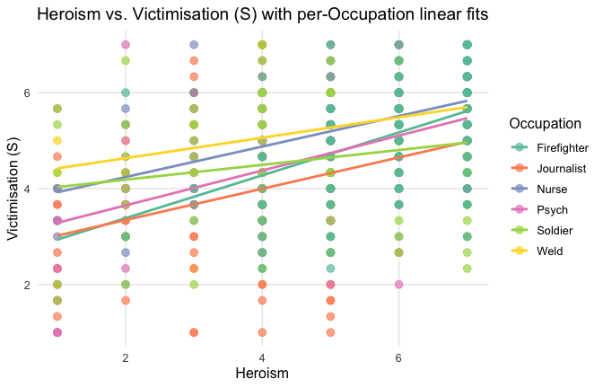

==> No support for our hypotheses. Across all occupations Heroism predicted POSITIVE general- and specific-level workers’ victimization, with or without controlling for attitude. Although effects were drastically reduced when accounting for attitude, heroism might increase our perception that workers need help and support, and suffer and are exploited. Our hypotheses should therefore be revised.

Model 1: “~Heroism + Occupation”

# =========================
# OLD MODELS (Heroism)
# =========================
m1_H <- lm(Victim_S_mean ~ Heroism + Occupation, data = scale_scores)
m2_H <- lm(Victim_S_mean ~ Heroism * Occupation, data = scale_scores)
m3_H <- lm(Victim_S_mean ~ Heroism + Occupation + Attitude, data = scale_scores)
m4_H <- lm(Victim_S_mean ~ Heroism * Occupation + Attitude, data = scale_scores)

tidy_type3(m1_H, "~Heroism + Cond")

~Heroism + Cond
	Term	df1	df2	F	p	eta2p
Heroism	Heroism	1	833	128.64	< .001	0.134
Occupation	Occupation	5	833	15.52	< .001	0.085

# =========================
# NEW MODELS (Danger & Help)
# =========================

Model 2: “~Heroism * Occupation”

tidy_type3(m2_H, "~Heroism * Cond")

~Heroism * Cond
	Term	df1	df2	F	p	eta2p
Heroism	Heroism	1	828	133.32	< .001	0.139
Occupation	Occupation	5	828	4.55	< .001	0.027
Heroism:Occupation	Heroism:Occupation	5	828	2.65	= 0.022	0.016

Model 3: “~Heroism + Occupation + Attitude”

tidy_type3(m3_H, "~Heroism + Occupation + Attitude")

~Heroism + Occupation + Attitude
	Term	df1	df2	F	p	eta2p
Heroism	Heroism	1	832	44.73	< .001	0.051
Occupation	Occupation	5	832	13.87	< .001	0.077
Attitude	Attitude	1	832	3.74	= 0.054	0.004

Model 4: “~Heroism * Occupation + Attitude”

tidy_type3(m4_H, "~Heroism * Occupation + Attitude")

~Heroism * Occupation + Attitude
	Term	df1	df2	F	p	eta2p
Heroism	Heroism	1	827	44.54	< .001	0.051
Occupation	Occupation	5	827	4.62	< .001	0.027
Attitude	Attitude	1	827	6.13	= 0.013	0.007
Heroism:Occupation	Heroism:Occupation	5	827	3.14	= 0.008	0.019

Comparison of main predictors across models

# Use orthogonal contrasts; keeps your "Heroism main effect" interpretable with Cond in the model
old_contr <- options(contrasts = c("contr.sum", "contr.poly"))

# Helper to extract the main effect of "Heroism" from a car::Anova table
extract_heroism <- function(mod, model_label) {
  a <- car::Anova(mod, type = "III")

  # Coerce to data.frame with rownames preserved
  tab <- as.data.frame(a)
  tab$Term <- rownames(tab)

  # Standard column names across R versions
  # (car::Anova uses these names for lm/glm type=III)
  # Columns: "Sum Sq", "Df", "F value", "Pr(>F)"
  names(tab) <- sub(" ", "_", names(tab))  # make names safe: "Sum_Sq", "F_value", etc.

  # Pull rows we need
  hero <- tab %>% filter(Term == "Heroism")
  resid <- tab %>% filter(Term == "Residuals")

  # Safety checks (in case of name variants)
  stopifnot(nrow(hero) == 1, nrow(resid) == 1)

  # Partial eta^2 = SS_effect / (SS_effect + SS_residual)
  eta_p2 <- hero$Sum_Sq / (hero$Sum_Sq + resid$Sum_Sq)

  # Format p nicely (APA-ish)
  p_fmt <- ifelse(hero$`Pr(>F)` < .001, "< .001",
                  sprintf("= %.3f", hero$`Pr(>F)`))

  dplyr::tibble(
    Model = model_label,
    Outcome = "Victim_S_mean",
    Predictor = "Heroism",
    df1 = hero$Df,
    df2 = resid$Df,
    F = hero$F_value,
    p = p_fmt,
    eta2p = eta_p2
  )
}

# ----- Fit the four models -----
mod1 <- lm(Victim_S_mean ~ Heroism + Cond, data = scale_scores)
mod2 <- lm(Victim_S_mean ~ Heroism * Cond, data = scale_scores)
mod3 <- lm(Victim_S_mean ~ Heroism + Cond + scale(Attitude), data = scale_scores)
mod4 <- lm(Victim_S_mean ~ Heroism * Cond + scale(Attitude), data = scale_scores)

# ----- Build the summary table -----
tbl <- bind_rows(
  extract_heroism(mod1, "~ Heroism + Cond"),
  extract_heroism(mod2, "~ Heroism * Occupation"),
  extract_heroism(mod3, "~ Heroism + Cond + Attitude"),
  extract_heroism(mod4, "~ Heroism * Occupation + Attitude")
  ) %>%
  # Nice number formatting for F and eta^2p
  mutate(
    F = round(F, 2),
    eta2p = round(eta2p, 3)
  )

# ----- Print as HTML-friendly table -----
# Build the table first
tbl_kbl <- tbl %>%
  kable("html",
        caption = "Main effect of Heroism across models (Type-III ANOVA): F, p, partial η²",
        align = "lllrrrcr")
# Add a footnote in a version-robust way
if ("footnote" %in% getNamespaceExports("kableExtra")) {
  tbl_kbl <- tbl_kbl %>%
    kableExtra::footnote(
      general = "Type-III sums of squares with sum contrasts. Partial η² = SS_effect / (SS_effect + SS_residual). p values are APA-style.",
      general_title = ""
    )
} else {
  tbl_kbl <- tbl_kbl %>%
    kableExtra::add_footnote(
      label = "Type-III sums of squares with sum contrasts. Partial η² = SS_effect / (SS_effect + SS_residual). p values are APA-style.",
      notation = "none"
    )
}

tbl_kbl

Main effect of Heroism across models (Type-III ANOVA): F, p, partial η²
Model	Outcome	Predictor	df1	df2	F	p	eta2p
~ Heroism + Cond	Victim_S_mean	Heroism	1	833	128.64	< .001	0.134
~ Heroism * Occupation	Victim_S_mean	Heroism	1	828	133.32	< .001	0.139
~ Heroism + Cond + Attitude	Victim_S_mean	Heroism	1	832	44.73	< .001	0.051
~ Heroism * Occupation + Attitude	Victim_S_mean	Heroism	1	827	44.54	< .001	0.051
Type-III sums of squares with sum contrasts. Partial η² = SS_effect / (SS_effect + SS_residual). p values are APA-style.

H5: Heroism is associated to greater impunity

Because Heroic status might also be incompatible with the villain status (Hartman et al., 2022), we should grant greater impunity to heroes, perceived as moral instances. At the general level, it means that we would support de-regulating the occupations. At the specific level, it means that in the context of a moral dilemma contrasting respecting the rules vs doing one’s job, we would be in favour of protecting rule-breaking heroes.

General level

Journalists should be given more freedom in the way they do their work

Toggle details of the models diagnostics and outlier analyses

Below, you’ll find model diagnostics (QQ plot, fitted vs residuals, linearity), Outliers analysis, and more details on the output

[NOTE THAT EFFECT SIZES REPORTED IN THE REPORT COMMANDS BELOW SHOULD NOT BE TRUSTED]

paste0("####################################################")

## [1] "####################################################"

paste0("Diagnostics for Model 1: DV ~ Heroism + Occupation")

## [1] "Diagnostics for Model 1: DV ~ Heroism + Occupation"

paste0("####################################################")

## [1] "####################################################"

mod1 <- lm(Villain_G_mean ~ Heroism  + Cond, data = scale_scores)
mod1r <- lmrob(Villain_G_mean ~ Heroism  + Cond, data = scale_scores)
plot(mod1)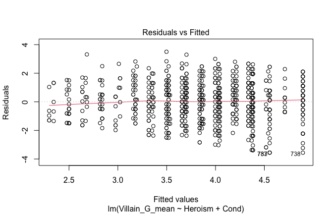

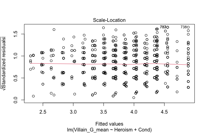
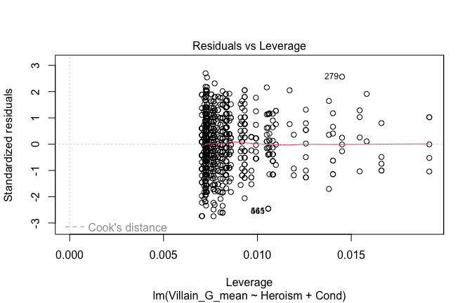
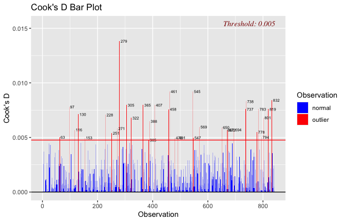
ols_plot_cooksd_bar(mod1, type = 1)

paste0("Comparison with Robust model")

## [1] "Comparison with Robust model"

models <- list("OLS (lm)" = mod1, "Robust (lmrob)" = mod1r)
modelsummary(
  models,
  statistic = c("({std.error})", "{statistic}", "p = {p.value}"),
  gof_omit  = "IC|Log.Lik",   # robust AIC comparability is iffy; omit by default
  output    = "html"
)

	OLS (lm)	Robust (lmrob)
(Intercept)	2.184	2.106
	(0.159)	(0.160)
	13.762	13.178
	p = <0.001	p = <0.001
Heroism	0.340	0.360
	(0.031)	(0.032)
	11.001	11.292
	p = <0.001	p = <0.001
Cond1	0.331	0.369
	(0.105)	(0.111)
	3.155	3.331
	p = 0.002	p = <0.001
Cond2	−0.024	−0.033
	(0.109)	(0.109)
	−0.220	−0.305
	p = 0.826	p = 0.761
Cond3	−0.181	−0.179
	(0.103)	(0.108)
	−1.763	−1.650
	p = 0.078	p = 0.099
Cond4	−0.046	−0.034
	(0.101)	(0.104)
	−0.453	−0.330
	p = 0.651	p = 0.741
Cond5	−0.227	−0.272
	(0.101)	(0.115)
	−2.243	−2.369
	p = 0.025	p = 0.018
Num.Obs.	840	840
R2	0.183	0.202
R2 Adj.	0.177	0.197
RMSE	1.30	1.30

fitted_vals <- fitted(mod1)

# Plot observed values against fitted values
plot(fitted_vals, scale_scores$Villain_G_mean,
     xlab = "Fitted Values",
     ylab = "Observed DV",
     main = "Observed vs Fitted Values")
abline(0, 1, col = "blue", lty = 2)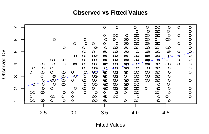

paste0("####################################################")

## [1] "####################################################"

paste0("Diagnostics for Model 2: DV ~ Heroism * Occupation")

## [1] "Diagnostics for Model 2: DV ~ Heroism * Occupation"

paste0("####################################################")

## [1] "####################################################"

mod1 <- lm(Villain_G_mean ~ Heroism  * Cond, data = scale_scores)
mod1r <- lmrob(Villain_G_mean ~ Heroism  * Cond, data = scale_scores)
plot(mod1)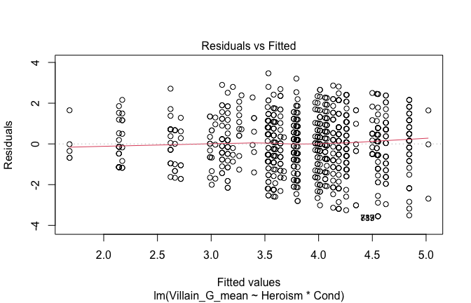

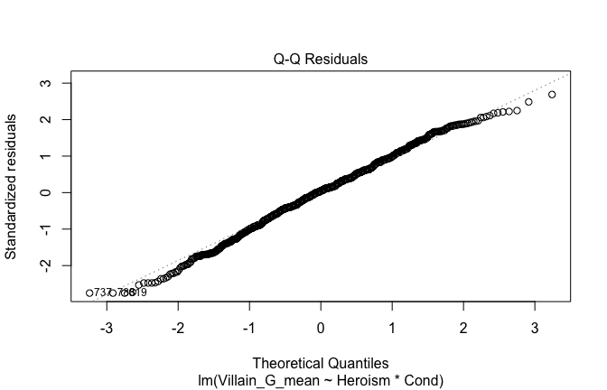
ols_plot_cooksd_bar(mod1, type = 1)

paste0("Comparison with Robust model")

## [1] "Comparison with Robust model"

models <- list("OLS (lm)" = mod1, "Robust (lmrob)" = mod1r)
modelsummary(
  models,
  statistic = c("({std.error})", "{statistic}", "p = {p.value}"),
  gof_omit  = "IC|Log.Lik",   # robust AIC comparability is iffy; omit by default
  output    = "html"
)

	OLS (lm)	Robust (lmrob)
(Intercept)	2.284	2.194
	(0.166)	(0.169)
	13.723	12.998
	p = <0.001	p = <0.001
Heroism	0.329	0.351
	(0.032)	(0.032)
	10.408	10.897
	p = <0.001	p = <0.001
Cond1	0.518	0.372
	(0.498)	(0.544)
	1.042	0.685
	p = 0.298	p = 0.494
Cond2	−0.622	−0.602
	(0.283)	(0.259)
	−2.199	−2.323
	p = 0.028	p = 0.020
Cond3	0.524	0.507
	(0.370)	(0.379)
	1.415	1.337
	p = 0.157	p = 0.182
Cond4	0.161	0.169
	(0.334)	(0.335)
	0.483	0.504
	p = 0.629	p = 0.614
Cond5	−1.093	−1.069
	(0.333)	(0.323)
	−3.283	−3.313
	p = 0.001	p = <0.001
Heroism × Cond1	−0.037	−0.006
	(0.084)	(0.091)
	−0.448	−0.061
	p = 0.654	p = 0.951
Heroism × Cond2	0.151	0.147
	(0.067)	(0.064)
	2.247	2.294
	p = 0.025	p = 0.022
Heroism × Cond3	−0.132	−0.129
	(0.065)	(0.068)
	−2.038	−1.903
	p = 0.042	p = 0.057
Heroism × Cond4	−0.057	−0.056
	(0.069)	(0.069)
	−0.833	−0.802
	p = 0.405	p = 0.423
Heroism × Cond5	0.162	0.151
	(0.063)	(0.064)
	2.585	2.374
	p = 0.010	p = 0.018
Num.Obs.	840	840
R2	0.198	0.218
R2 Adj.	0.187	0.207
RMSE	1.29	1.29

fitted_vals <- fitted(mod1)

# Plot observed values against fitted values
plot(fitted_vals, scale_scores$Villain_G_mean,
     xlab = "Fitted Values",
     ylab = "Observed DV",
     main = "Observed vs Fitted Values")
abline(0, 1, col = "blue", lty = 2)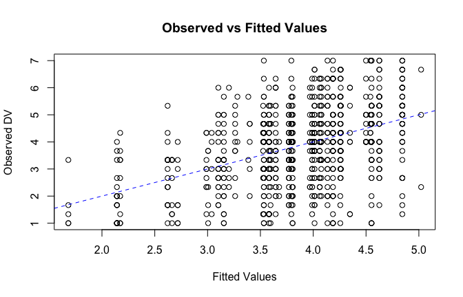

paste0("####################################################")

## [1] "####################################################"

paste0("Diagnostics for Model 3: DV ~ Heroism + Occupation + Attitude")

## [1] "Diagnostics for Model 3: DV ~ Heroism + Occupation + Attitude"

paste0("####################################################")

## [1] "####################################################"

mod1 <- lm(Villain_G_mean ~ Heroism  + Cond + Attitude, data = scale_scores)
mod1r <- lmrob(Villain_G_mean ~ Heroism  + Cond + Attitude, data = scale_scores)
plot(mod1)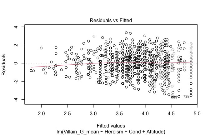

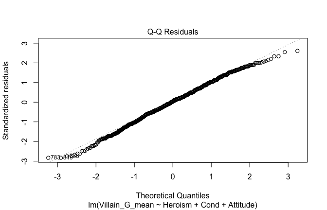
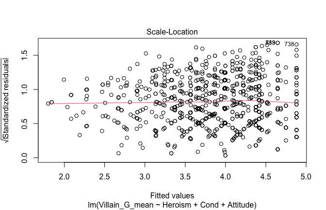
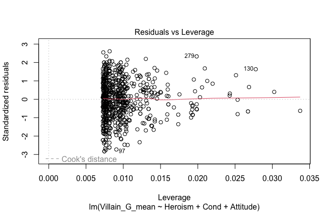
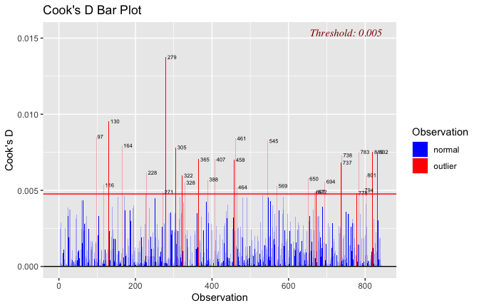
ols_plot_cooksd_bar(mod1, type = 1)

paste0("Comparison with Robust model")

## [1] "Comparison with Robust model"

models <- list("OLS (lm)" = mod1, "Robust (lmrob)" = mod1r)
modelsummary(
  models,
  statistic = c("({std.error})", "{statistic}", "p = {p.value}"),
  gof_omit  = "IC|Log.Lik",   # robust AIC comparability is iffy; omit by default
  output    = "html"
)

	OLS (lm)	Robust (lmrob)
(Intercept)	2.708	2.618
	(0.218)	(0.217)
	12.420	12.047
	p = <0.001	p = <0.001
Heroism	0.234	0.257
	(0.043)	(0.043)
	5.393	5.935
	p = <0.001	p = <0.001
Cond1	0.277	0.322
	(0.105)	(0.112)
	2.634	2.862
	p = 0.009	p = 0.004
Cond2	0.058	0.044
	(0.111)	(0.109)
	0.526	0.400
	p = 0.599	p = 0.689
Cond3	−0.227	−0.223
	(0.103)	(0.109)
	−2.212	−2.041
	p = 0.027	p = 0.042
Cond4	−0.071	−0.065
	(0.101)	(0.104)
	−0.707	−0.621
	p = 0.480	p = 0.535
Cond5	−0.183	−0.230
	(0.101)	(0.113)
	−1.806	−2.034
	p = 0.071	p = 0.042
Attitude	0.253	0.242
	(0.073)	(0.070)
	3.480	3.478
	p = <0.001	p = <0.001
Num.Obs.	840	840
R2	0.194	0.213
R2 Adj.	0.187	0.206
RMSE	1.29	1.29

fitted_vals <- fitted(mod1)

# Plot observed values against fitted values
plot(fitted_vals, scale_scores$Villain_G_mean,
     xlab = "Fitted Values",
     ylab = "Observed DV",
     main = "Observed vs Fitted Values")
abline(0, 1, col = "blue", lty = 2)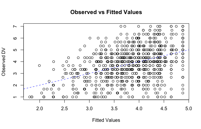

paste0("####################################################")

## [1] "####################################################"

paste0("Diagnostics for Model 4: DV ~ Heroism * Occupation + Attitude")

## [1] "Diagnostics for Model 4: DV ~ Heroism * Occupation + Attitude"

paste0("####################################################")

## [1] "####################################################"

mod1 <- lm(Villain_G_mean ~ Heroism*Cond + Attitude, data = scale_scores)
mod1r <- lmrob(Villain_G_mean ~ Heroism*Cond + Attitude, data = scale_scores)
plot(mod1)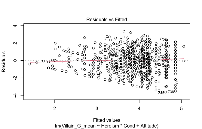

ols_plot_cooksd_bar(mod1, type = 1)

paste0("Comparison with Robust model")

## [1] "Comparison with Robust model"

models <- list("OLS (lm)" = mod1, "Robust (lmrob)" = mod1r)
modelsummary(
  models,
  statistic = c("({std.error})", "{statistic}", "p = {p.value}"),
  gof_omit  = "IC|Log.Lik",   # robust AIC comparability is iffy; omit by default
  output    = "html"
)

	OLS (lm)	Robust (lmrob)
(Intercept)	2.690	2.593
	(0.220)	(0.227)
	12.203	11.424
	p = <0.001	p = <0.001
Heroism	0.245	0.269
	(0.044)	(0.044)
	5.637	6.081
	p = <0.001	p = <0.001
Cond1	0.355	0.238
	(0.499)	(0.538)
	0.712	0.443
	p = 0.476	p = 0.658
Cond2	−0.461	−0.455
	(0.288)	(0.258)
	−1.602	−1.764
	p = 0.110	p = 0.078
Cond3	0.465	0.442
	(0.370)	(0.369)
	1.258	1.197
	p = 0.209	p = 0.232
Cond4	0.094	0.087
	(0.334)	(0.341)
	0.283	0.254
	p = 0.777	p = 0.800
Cond5	−0.907	−0.877
	(0.338)	(0.310)
	−2.682	−2.828
	p = 0.007	p = 0.005
Attitude	0.207	0.198
	(0.074)	(0.071)
	2.793	2.777
	p = 0.005	p = 0.006
Heroism × Cond1	−0.017	0.011
	(0.084)	(0.090)
	−0.201	0.123
	p = 0.841	p = 0.902
Heroism × Cond2	0.128	0.126
	(0.067)	(0.063)
	1.896	1.983
	p = 0.058	p = 0.048
Heroism × Cond3	−0.127	−0.124
	(0.065)	(0.066)
	−1.973	−1.863
	p = 0.049	p = 0.063
Heroism × Cond4	−0.045	−0.041
	(0.069)	(0.070)
	−0.656	−0.585
	p = 0.512	p = 0.559
Heroism × Cond5	0.133	0.122
	(0.063)	(0.062)
	2.117	1.971
	p = 0.035	p = 0.049
Num.Obs.	840	840
R2	0.205	0.224
R2 Adj.	0.194	0.212
RMSE	1.28	1.28

fitted_vals <- fitted(mod1)

# Plot observed values against fitted values
plot(fitted_vals, scale_scores$Villain_G_mean,
     xlab = "Fitted Values",
     ylab = "Observed DV",
     main = "Observed vs Fitted Values")
abline(0, 1, col = "blue", lty = 2)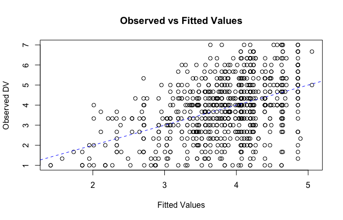

paste0("####################################################")

## [1] "####################################################"

paste0("REPORTS for each model (please ignore the eta squares, they are way off")

## [1] "REPORTS for each model (please ignore the eta squares, they are way off"

paste0("####################################################")

## [1] "####################################################"

paste0("MODEL 1: Villain_G_mean ~ Heroism")

## [1] "MODEL 1: Villain_G_mean ~ Heroism"

report(Anova(mod1 <- lm(Villain_G_mean ~ Heroism  + Cond, data = scale_scores), type = "III"))

## The ANOVA suggests that:
## 
##   - The main effect of Heroism is statistically significant and medium (F(1, 833)
## = 121.02, p < .001; Eta2 (partial) = 0.13, 95% CI [0.09, 1.00])
##   - The main effect of Cond is statistically significant and small (F(5, 833) =
## 3.56, p = 0.003; Eta2 (partial) = 0.02, 95% CI [4.13e-03, 1.00])
## 
## Effect sizes were labelled following Field's (2013) recommendations.

paste0("MODEL 2: Villain_G_mean ~ Heroism * Cond")

## [1] "MODEL 2: Villain_G_mean ~ Heroism * Cond"

report(Anova(mod2 <- lm(Villain_G_mean ~ Heroism * Cond, data = scale_scores), type = "III"))

## Type 3 ANOVAs only give sensible and informative results when covariates
##   are mean-centered and factors are coded with orthogonal contrasts (such
##   as those produced by `contr.sum`, `contr.poly`, or `contr.helmert`, but
##   *not* by the default `contr.treatment`).

## The ANOVA suggests that:
## 
##   - The main effect of Heroism is statistically significant and medium (F(1, 828)
## = 108.33, p < .001; Eta2 (partial) = 0.12, 95% CI [0.08, 1.00])
##   - The main effect of Cond is statistically significant and small (F(5, 828) =
## 3.47, p = 0.004; Eta2 (partial) = 0.02, 95% CI [3.85e-03, 1.00])
##   - The interaction between Heroism and Cond is statistically significant and
## small (F(5, 828) = 3.12, p = 0.008; Eta2 (partial) = 0.02, 95% CI [2.69e-03,
## 1.00])
## 
## Effect sizes were labelled following Field's (2013) recommendations.

paste0("MODEL 3: Villain_G_mean ~ Heroism +scale(Attitude)")

## [1] "MODEL 3: Villain_G_mean ~ Heroism +scale(Attitude)"

report(Anova(mod3 <- lm(Villain_G_mean ~ Heroism   + Cond +scale(Attitude) , data = scale_scores), type = "III"))

## The ANOVA suggests that:
## 
##   - The main effect of Heroism is statistically significant and small (F(1, 832)
## = 29.09, p < .001; Eta2 (partial) = 0.03, 95% CI [0.02, 1.00])
##   - The main effect of Cond is statistically significant and small (F(5, 832) =
## 3.21, p = 0.007; Eta2 (partial) = 0.02, 95% CI [2.98e-03, 1.00])
##   - The main effect of scale(Attitude) is statistically significant and small
## (F(1, 832) = 12.11, p < .001; Eta2 (partial) = 0.01, 95% CI [4.00e-03, 1.00])
## 
## Effect sizes were labelled following Field's (2013) recommendations.

paste0("MODEL 4: Villain_G_mean ~ Heroism * Cond + scale(Attitude)")

## [1] "MODEL 4: Villain_G_mean ~ Heroism * Cond + scale(Attitude)"

report(Anova(mod4 <-lm(Villain_G_mean ~ Heroism * Cond + scale(Attitude), data = scale_scores), type = "III"))

## Type 3 ANOVAs only give sensible and informative results when covariates
##   are mean-centered and factors are coded with orthogonal contrasts (such
##   as those produced by `contr.sum`, `contr.poly`, or `contr.helmert`, but
##   *not* by the default `contr.treatment`).

## The ANOVA suggests that:
## 
##   - The main effect of Heroism is statistically significant and small (F(1, 827)
## = 31.78, p < .001; Eta2 (partial) = 0.04, 95% CI [0.02, 1.00])
##   - The main effect of Cond is statistically not significant and small (F(5, 827)
## = 2.15, p = 0.058; Eta2 (partial) = 0.01, 95% CI [0.00, 1.00])
##   - The main effect of scale(Attitude) is statistically significant and very
## small (F(1, 827) = 7.80, p = 0.005; Eta2 (partial) = 9.34e-03, 95% CI
## [1.58e-03, 1.00])
##   - The interaction between Heroism and Cond is statistically significant and
## small (F(5, 827) = 2.27, p = 0.046; Eta2 (partial) = 0.01, 95% CI [1.15e-04,
## 1.00])
## 
## Effect sizes were labelled following Field's (2013) recommendations.

paste0("Model Comparison: assessing the importance of attitude - not accounting for occupations")

## [1] "Model Comparison: assessing the importance of attitude - not accounting for occupations"

anova(mod1, mod3)

paste0("Model Comparison: assessing the importance of attitude - accounting for occupations")

## [1] "Model Comparison: assessing the importance of attitude - accounting for occupations"

anova(mod2, mod4)

ggplot(scale_scores, aes(y = Villain_G_mean, x = Heroism)) +
  # 1) points colored by Cond
  geom_point(aes(color = Cond),
             size = 2.7, alpha = 0.7) +
  
  # 2) ONE global lm line (group = 1 prevents one line per Cond)
  stat_smooth(method = "lm", se = TRUE,
              aes(group = 1),
              color = "black", linewidth = 1) +
  
  # Nice, accessible palette (works well with >3 groups)
  scale_color_brewer(palette = "Set2") +
  
  labs(
    y = "Impunity (G)",
    x = "Heroism",
    color = "Occupation",
    title = "Heroism vs. Impunity (G), colored by Occupation",
    subtitle = "Points are participants; black line is overall linear fit with 95% CI"
  ) +
  theme_minimal(base_size = 12) +
  theme(
    legend.position = "right",
    panel.grid.minor = element_blank()
  )

## `geom_smooth()` using formula = 'y ~ x'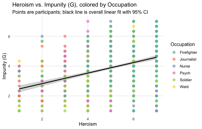

ggplot(scale_scores, aes(y = Villain_G_mean, x = Heroism, color = Cond)) +
  # points colored by condition
  geom_point(size = 2.7, alpha = 0.7) +
  # ONE lm line PER condition (because color is mapped here)
  stat_smooth(method = "lm", se = FALSE, linewidth = 1, fullrange = TRUE) +
  scale_color_brewer(palette = "Set2") +
  labs(
    y = "Impunity (G) ",
    x = "Heroism",
    color = "Occupation",
    title = "Heroism vs. Impunity (G) with per-Occupation linear fits"
  ) +
  theme_minimal(base_size = 12) +
  theme(legend.position = "right", panel.grid.minor = element_blank())

## `geom_smooth()` using formula = 'y ~ x'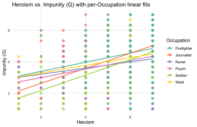

Model 1: “~Heroism + Occupation”

# =========================
# OLD MODELS (Heroism)
# =========================
m1_H <- lm(Villain_G_mean ~ Heroism + Occupation, data = scale_scores)
m2_H <- lm(Villain_G_mean ~ Heroism * Occupation, data = scale_scores)
m3_H <- lm(Villain_G_mean ~ Heroism + Occupation + Attitude, data = scale_scores)
m4_H <- lm(Villain_G_mean ~ Heroism * Occupation + Attitude, data = scale_scores)

tidy_type3(m1_H, "~Heroism + Cond")

~Heroism + Cond
	Term	df1	df2	F	p	eta2p
Heroism	Heroism	1	833	121.02	< .001	0.127
Occupation	Occupation	5	833	3.56	= 0.003	0.021

# =========================
# NEW MODELS (Danger & Help)
# =========================

Model 2: “~Heroism * Occupation”

tidy_type3(m2_H, "~Heroism * Cond")

~Heroism * Cond
	Term	df1	df2	F	p	eta2p
Heroism	Heroism	1	828	108.33	< .001	0.116
Occupation	Occupation	5	828	3.47	= 0.004	0.021
Heroism:Occupation	Heroism:Occupation	5	828	3.12	= 0.008	0.019

Model 3: “~Heroism + Occupation + Attitude”

tidy_type3(m3_H, "~Heroism + Occupation + Attitude")

~Heroism + Occupation + Attitude
	Term	df1	df2	F	p	eta2p
Heroism	Heroism	1	832	29.09	< .001	0.034
Occupation	Occupation	5	832	3.21	= 0.007	0.019
Attitude	Attitude	1	832	12.11	< .001	0.014

Model 4: “~Heroism * Occupation + Attitude”

tidy_type3(m4_H, "~Heroism * Occupation + Attitude")

~Heroism * Occupation + Attitude
	Term	df1	df2	F	p	eta2p
Heroism	Heroism	1	827	31.78	< .001	0.037
Occupation	Occupation	5	827	2.15	= 0.058	0.013
Attitude	Attitude	1	827	7.80	= 0.005	0.009
Heroism:Occupation	Heroism:Occupation	5	827	2.27	= 0.046	0.014

Comparison of main predictors across models

# Use orthogonal contrasts; keeps your "Heroism main effect" interpretable with Cond in the model
old_contr <- options(contrasts = c("contr.sum", "contr.poly"))

# Helper to extract the main effect of "Heroism" from a car::Anova table
extract_heroism <- function(mod, model_label) {
  a <- car::Anova(mod, type = "III")

  # Coerce to data.frame with rownames preserved
  tab <- as.data.frame(a)
  tab$Term <- rownames(tab)

  # Standard column names across R versions
  # (car::Anova uses these names for lm/glm type=III)
  # Columns: "Sum Sq", "Df", "F value", "Pr(>F)"
  names(tab) <- sub(" ", "_", names(tab))  # make names safe: "Sum_Sq", "F_value", etc.

  # Pull rows we need
  hero <- tab %>% filter(Term == "Heroism")
  resid <- tab %>% filter(Term == "Residuals")

  # Safety checks (in case of name variants)
  stopifnot(nrow(hero) == 1, nrow(resid) == 1)

  # Partial eta^2 = SS_effect / (SS_effect + SS_residual)
  eta_p2 <- hero$Sum_Sq / (hero$Sum_Sq + resid$Sum_Sq)

  # Format p nicely (APA-ish)
  p_fmt <- ifelse(hero$`Pr(>F)` < .001, "< .001",
                  sprintf("= %.3f", hero$`Pr(>F)`))

  dplyr::tibble(
    Model = model_label,
    Outcome = "Villain_G_mean",
    Predictor = "Heroism",
    df1 = hero$Df,
    df2 = resid$Df,
    F = hero$F_value,
    p = p_fmt,
    eta2p = eta_p2
  )
}

# ----- Fit the four models -----
mod1 <- lm(Villain_G_mean ~ Heroism + Cond, data = scale_scores)
mod2 <- lm(Villain_G_mean ~ Heroism * Cond, data = scale_scores)
mod3 <- lm(Villain_G_mean ~ Heroism + Cond + scale(Attitude), data = scale_scores)
mod4 <- lm(Villain_G_mean ~ Heroism * Cond + scale(Attitude), data = scale_scores)

# ----- Build the summary table -----
tbl <- bind_rows(
  extract_heroism(mod1, "~ Heroism + Cond"),
  extract_heroism(mod2, "~ Heroism * Occupation"),
  extract_heroism(mod3, "~ Heroism + Cond + Attitude"),
  extract_heroism(mod4, "~ Heroism * Occupation + Attitude")
  ) %>%
  # Nice number formatting for F and eta^2p
  mutate(
    F = round(F, 2),
    eta2p = round(eta2p, 3)
  )

# ----- Print as HTML-friendly table -----
# Build the table first
tbl_kbl <- tbl %>%
  kable("html",
        caption = "Main effect of Heroism across models (Type-III ANOVA): F, p, partial η²",
        align = "lllrrrcr")
# Add a footnote in a version-robust way
if ("footnote" %in% getNamespaceExports("kableExtra")) {
  tbl_kbl <- tbl_kbl %>%
    kableExtra::footnote(
      general = "Type-III sums of squares with sum contrasts. Partial η² = SS_effect / (SS_effect + SS_residual). p values are APA-style.",
      general_title = ""
    )
} else {
  tbl_kbl <- tbl_kbl %>%
    kableExtra::add_footnote(
      label = "Type-III sums of squares with sum contrasts. Partial η² = SS_effect / (SS_effect + SS_residual). p values are APA-style.",
      notation = "none"
    )
}

tbl_kbl

Main effect of Heroism across models (Type-III ANOVA): F, p, partial η²
Model	Outcome	Predictor	df1	df2	F	p	eta2p
~ Heroism + Cond	Villain_G_mean	Heroism	1	833	121.02	< .001	0.127
~ Heroism * Occupation	Villain_G_mean	Heroism	1	828	108.33	< .001	0.116
~ Heroism + Cond + Attitude	Villain_G_mean	Heroism	1	832	29.09	< .001	0.034
~ Heroism * Occupation + Attitude	Villain_G_mean	Heroism	1	827	31.78	< .001	0.037
Type-III sums of squares with sum contrasts. Partial η² = SS_effect / (SS_effect + SS_residual). p values are APA-style.

Specific level

UK journalists must follow strict codes of ethics, such as IPSO rules and their employers’ policies. These ban phone hacking or wiretapping except in rare, extreme cases. The rules stress respect for privacy, following the law, and avoiding unjustified intrusion, even for the public interest. A national journalist suspects a top official of abusing their position by steering public contracts to companies owned by close associates, raising concerns of corruption and misuse of public money. With no evidence and official investigations blocked, the journalist believes normal reporting won’t work fast enough. They secretly tap the phones of the official, his wife, and two daughters for several weeks, hoping to find proof.

Toggle details of the models diagnostics and outlier analyses

Below, you’ll find model diagnostics (QQ plot, fitted vs residuals, linearity), Outliers analysis, and more details on the output

[NOTE THAT EFFECT SIZES REPORTED IN THE REPORT COMMANDS BELOW SHOULD NOT BE TRUSTED]

paste0("####################################################")

## [1] "####################################################"

paste0("Diagnostics for Model 1: DV ~ Heroism + Occupation")

## [1] "Diagnostics for Model 1: DV ~ Heroism + Occupation"

paste0("####################################################")

## [1] "####################################################"

mod1 <- lm(Villain_S_mean ~ Heroism  + Cond, data = scale_scores)
mod1r <- lmrob(Villain_S_mean ~ Heroism  + Cond, data = scale_scores)
plot(mod1)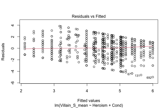

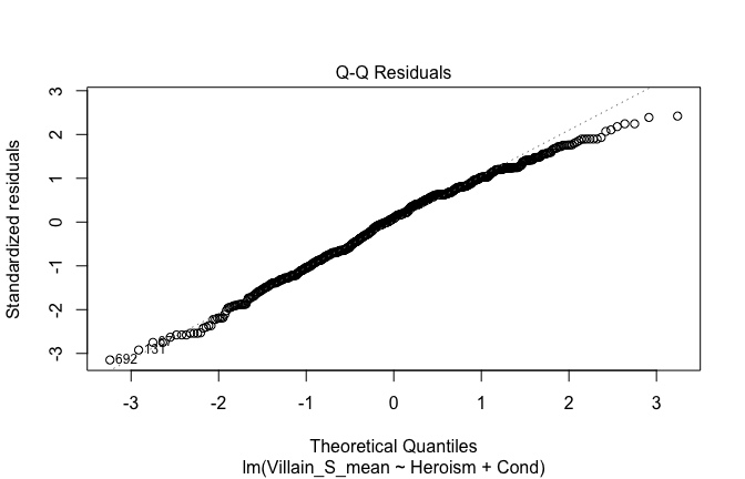
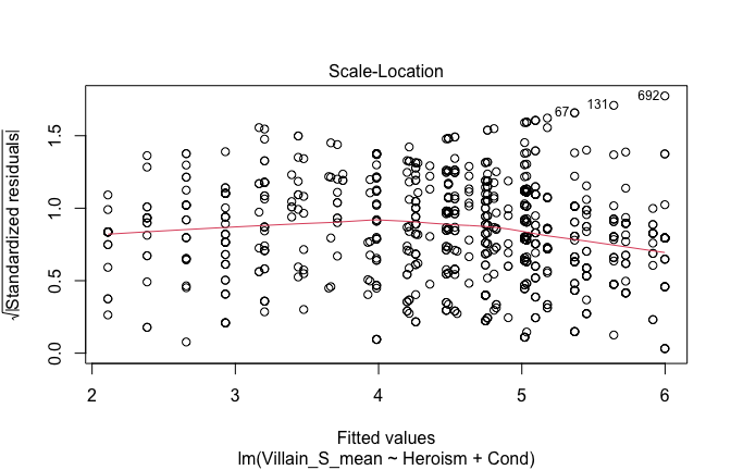
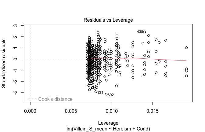
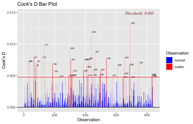
ols_plot_cooksd_bar(mod1, type = 1)

paste0("Comparison with Robust model")

## [1] "Comparison with Robust model"

models <- list("OLS (lm)" = mod1, "Robust (lmrob)" = mod1r)
modelsummary(
  models,
  statistic = c("({std.error})", "{statistic}", "p = {p.value}"),
  gof_omit  = "IC|Log.Lik",   # robust AIC comparability is iffy; omit by default
  output    = "html"
)

	OLS (lm)	Robust (lmrob)
(Intercept)	3.174	3.055
	(0.194)	(0.224)
	16.337	13.637
	p = <0.001	p = <0.001
Heroism	0.273	0.309
	(0.038)	(0.043)
	7.227	7.129
	p = <0.001	p = <0.001
Cond1	−0.068	−0.114
	(0.128)	(0.120)
	−0.529	−0.949
	p = 0.597	p = 0.343
Cond2	−1.336	−1.413
	(0.133)	(0.150)
	−10.012	−9.392
	p = <0.001	p = <0.001
Cond3	−0.053	−0.010
	(0.126)	(0.169)
	−0.425	−0.058
	p = 0.671	p = 0.954
Cond4	−0.281	−0.344
	(0.124)	(0.161)
	−2.274	−2.136
	p = 0.023	p = 0.033
Cond5	0.911	0.951
	(0.124)	(0.108)
	7.354	8.822
	p = <0.001	p = <0.001
Num.Obs.	840	840
R2	0.271	0.311
R2 Adj.	0.266	0.306
RMSE	1.59	1.59

fitted_vals <- fitted(mod1)

# Plot observed values against fitted values
plot(fitted_vals, scale_scores$Villain_S_mean,
     xlab = "Fitted Values",
     ylab = "Observed DV",
     main = "Observed vs Fitted Values")
abline(0, 1, col = "blue", lty = 2)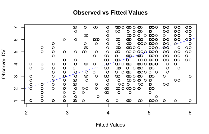

paste0("####################################################")

## [1] "####################################################"

paste0("Diagnostics for Model 2: DV ~ Heroism * Occupation")

## [1] "Diagnostics for Model 2: DV ~ Heroism * Occupation"

paste0("####################################################")

## [1] "####################################################"

mod1 <- lm(Villain_S_mean ~ Heroism  * Cond, data = scale_scores)
mod1r <- lmrob(Villain_S_mean ~ Heroism  * Cond, data = scale_scores)

## Warning in lmrob.S(x, y, control = control): S refinements did not converge (to
## refine.tol=1e-07) in 200 (= k.max) steps

## Warning in lmrob.fit(x, y, control, init = init): initial estim. 'init' not
## converged -- will be return()ed basically unchanged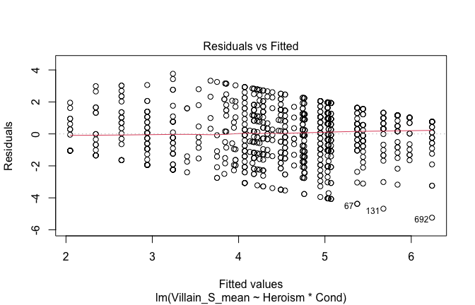

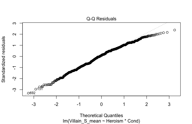
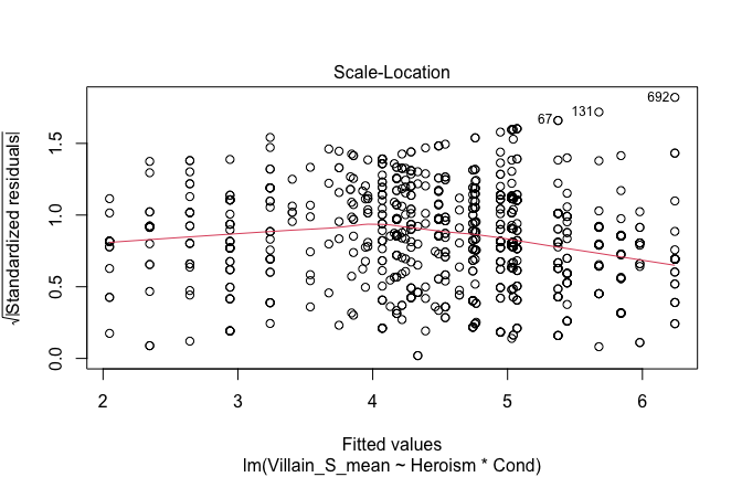
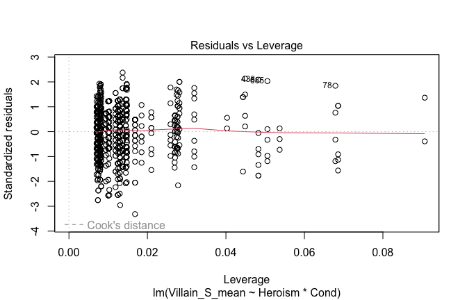
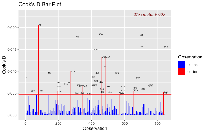
plot(mod1)

ols_plot_cooksd_bar(mod1, type = 1)

paste0("Comparison with Robust model")

## [1] "Comparison with Robust model"

models <- list("OLS (lm)" = mod1, "Robust (lmrob)" = mod1r)
modelsummary(
  models,
  statistic = c("({std.error})", "{statistic}", "p = {p.value}"),
  gof_omit  = "IC|Log.Lik",   # robust AIC comparability is iffy; omit by default
  output    = "html"
)

	OLS (lm)	Robust (lmrob)
(Intercept)	3.224	2.463
	(0.205)
	15.734
	p = <0.001
Heroism	0.264	0.477
	(0.039)
	6.779
	p = <0.001
Cond1	0.293	−0.430
	(0.613)
	0.478
	p = 0.632
Cond2	−1.474	−1.456
	(0.348)
	−4.230
	p = <0.001
Cond3	−0.092	1.908
	(0.456)
	−0.202
	p = 0.840
Cond4	0.419	−1.949
	(0.411)
	1.020
	p = 0.308
Cond5	0.220	0.064
	(0.410)
	0.537
	p = 0.591
Heroism × Cond1	−0.060	0.034
	(0.103)
	−0.579
	p = 0.563
Heroism × Cond2	0.034	−0.180
	(0.083)
	0.410
	p = 0.682
Heroism × Cond3	0.007	−0.165
	(0.080)
	0.093
	p = 0.926
Heroism × Cond4	−0.157	0.324
	(0.085)
	−1.853
	p = 0.064
Heroism × Cond5	0.136	0.142
	(0.077)
	1.762
	p = 0.078
Num.Obs.	840	840
R2	0.276	0.798
R2 Adj.	0.267	0.795
RMSE	1.58	1.80

fitted_vals <- fitted(mod1)

# Plot observed values against fitted values
plot(fitted_vals, scale_scores$Villain_S_mean,
     xlab = "Fitted Values",
     ylab = "Observed DV",
     main = "Observed vs Fitted Values")
abline(0, 1, col = "blue", lty = 2)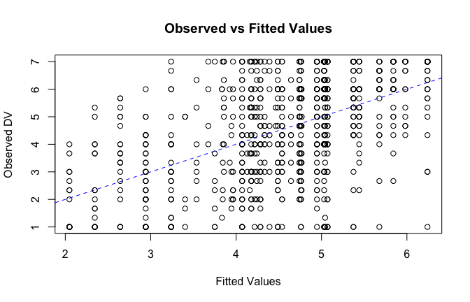

paste0("####################################################")

## [1] "####################################################"

paste0("Diagnostics for Model 3: DV ~ Heroism + Occupation + Attitude")

## [1] "Diagnostics for Model 3: DV ~ Heroism + Occupation + Attitude"

paste0("####################################################")

## [1] "####################################################"

mod1 <- lm(Villain_S_mean ~ Heroism  + Cond + Attitude, data = scale_scores)
mod1r <- lmrob(Villain_S_mean ~ Heroism  + Cond + Attitude, data = scale_scores)
plot(mod1)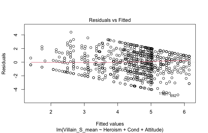

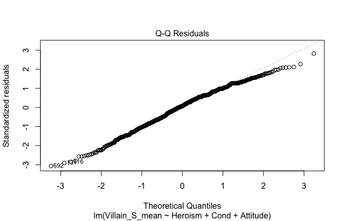
ols_plot_cooksd_bar(mod1, type = 1)

paste0("Comparison with Robust model")

## [1] "Comparison with Robust model"

models <- list("OLS (lm)" = mod1, "Robust (lmrob)" = mod1r)
modelsummary(
  models,
  statistic = c("({std.error})", "{statistic}", "p = {p.value}"),
  gof_omit  = "IC|Log.Lik",   # robust AIC comparability is iffy; omit by default
  output    = "html"
)

	OLS (lm)	Robust (lmrob)
(Intercept)	4.078	3.974
	(0.265)	(0.303)
	15.390	13.112
	p = <0.001	p = <0.001
Heroism	0.090	0.123
	(0.053)	(0.060)
	1.707	2.059
	p = 0.088	p = 0.040
Cond1	−0.160	−0.199
	(0.128)	(0.121)
	−1.253	−1.652
	p = 0.211	p = 0.099
Cond2	−1.195	−1.269
	(0.135)	(0.149)
	−8.865	−8.513
	p = <0.001	p = <0.001
Cond3	−0.134	−0.085
	(0.125)	(0.166)
	−1.071	−0.511
	p = 0.285	p = 0.609
Cond4	−0.325	−0.377
	(0.122)	(0.155)
	−2.659	−2.441
	p = 0.008	p = 0.015
Cond5	0.987	1.021
	(0.123)	(0.104)
	8.015	9.854
	p = <0.001	p = <0.001
Attitude	0.436	0.436
	(0.088)	(0.092)
	4.942	4.742
	p = <0.001	p = <0.001
Num.Obs.	840	840
R2	0.292	0.327
R2 Adj.	0.286	0.322
RMSE	1.57	1.57

fitted_vals <- fitted(mod1)

# Plot observed values against fitted values
plot(fitted_vals, scale_scores$Villain_S_mean,
     xlab = "Fitted Values",
     ylab = "Observed DV",
     main = "Observed vs Fitted Values")
abline(0, 1, col = "blue", lty = 2)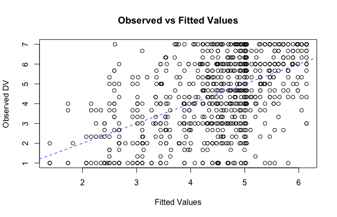

paste0("####################################################")

## [1] "####################################################"

paste0("Diagnostics for Model 4: DV ~ Heroism * Occupation + Attitude")

## [1] "Diagnostics for Model 4: DV ~ Heroism * Occupation + Attitude"

paste0("####################################################")

## [1] "####################################################"

mod1 <- lm(Villain_S_mean ~ Heroism*Cond + Attitude, data = scale_scores)
mod1r <- lmrob(Villain_S_mean ~ Heroism*Cond + Attitude, data = scale_scores)
plot(mod1)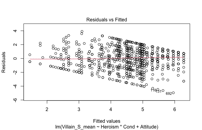

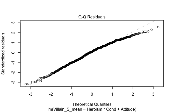
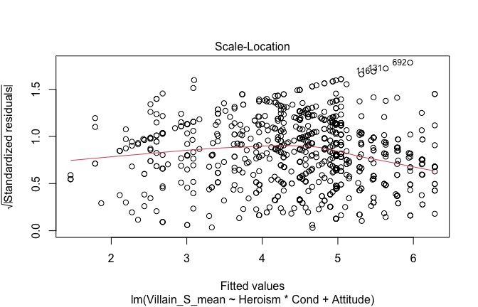
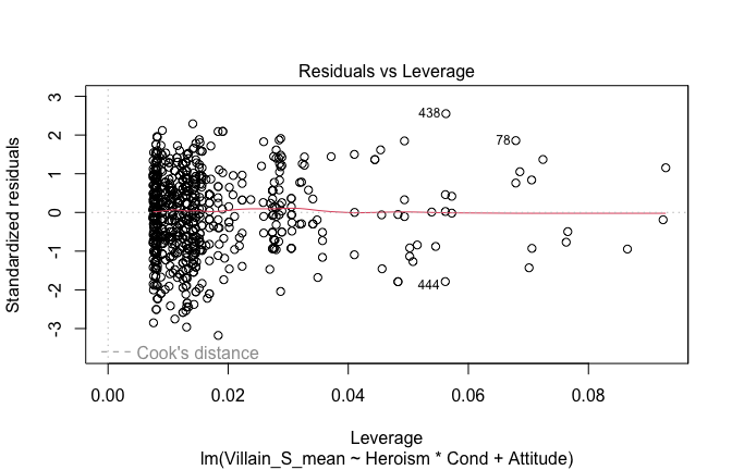
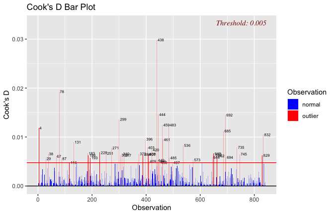
ols_plot_cooksd_bar(mod1, type = 1)

paste0("Comparison with Robust model")

## [1] "Comparison with Robust model"

models <- list("OLS (lm)" = mod1, "Robust (lmrob)" = mod1r)
modelsummary(
  models,
  statistic = c("({std.error})", "{statistic}", "p = {p.value}"),
  gof_omit  = "IC|Log.Lik",   # robust AIC comparability is iffy; omit by default
  output    = "html"
)

	OLS (lm)	Robust (lmrob)
(Intercept)	4.048	3.969
	(0.269)	(0.312)
	15.041	12.735
	p = <0.001	p = <0.001
Heroism	0.094	0.119
	(0.053)	(0.062)
	1.761	1.934
	p = 0.079	p = 0.054
Cond1	−0.038	−0.109
	(0.609)	(0.547)
	−0.062	−0.199
	p = 0.951	p = 0.843
Cond2	−1.146	−1.102
	(0.351)	(0.353)
	−3.261	−3.125
	p = 0.001	p = 0.002
Cond3	−0.213	−0.275
	(0.451)	(0.546)
	−0.471	−0.505
	p = 0.638	p = 0.614
Cond4	0.283	0.198
	(0.407)	(0.662)
	0.695	0.299
	p = 0.487	p = 0.765
Cond5	0.598	0.579
	(0.413)	(0.409)
	1.448	1.416
	p = 0.148	p = 0.157
Attitude	0.421	0.423
	(0.091)	(0.096)
	4.646	4.397
	p = <0.001	p = <0.001
Heroism × Cond1	−0.018	−0.009
	(0.102)	(0.094)
	−0.172	−0.099
	p = 0.864	p = 0.921
Heroism × Cond2	−0.013	−0.047
	(0.082)	(0.088)
	−0.158	−0.539
	p = 0.874	p = 0.590
Heroism × Cond3	0.017	0.040
	(0.079)	(0.094)
	0.216	0.423
	p = 0.829	p = 0.672
Heroism × Cond4	−0.132	−0.120
	(0.084)	(0.133)
	−1.576	−0.901
	p = 0.115	p = 0.368
Heroism × Cond5	0.079	0.091
	(0.077)	(0.073)
	1.020	1.240
	p = 0.308	p = 0.215
Num.Obs.	840	840
R2	0.295	0.331
R2 Adj.	0.284	0.321
RMSE	1.56	1.57

fitted_vals <- fitted(mod1)

# Plot observed values against fitted values
plot(fitted_vals, scale_scores$Villain_S_mean,
     xlab = "Fitted Values",
     ylab = "Observed DV",
     main = "Observed vs Fitted Values")
abline(0, 1, col = "blue", lty = 2)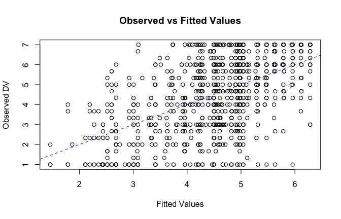

paste0("####################################################")

## [1] "####################################################"

paste0("REPORTS for each model (please ignore the eta squares, they are way off")

## [1] "REPORTS for each model (please ignore the eta squares, they are way off"

paste0("####################################################")

## [1] "####################################################"

paste0("MODEL 1: Villain_S_mean ~ Heroism")

## [1] "MODEL 1: Villain_S_mean ~ Heroism"

report(Anova(mod1 <- lm(Villain_S_mean ~ Heroism  + Cond, data = scale_scores), type = "III"))

## The ANOVA suggests that:
## 
##   - The main effect of Heroism is statistically significant and small (F(1, 833)
## = 52.23, p < .001; Eta2 (partial) = 0.06, 95% CI [0.04, 1.00])
##   - The main effect of Cond is statistically significant and large (F(5, 833) =
## 34.66, p < .001; Eta2 (partial) = 0.17, 95% CI [0.13, 1.00])
## 
## Effect sizes were labelled following Field's (2013) recommendations.

paste0("MODEL 2: Villain_S_mean ~ Heroism * Cond")

## [1] "MODEL 2: Villain_S_mean ~ Heroism * Cond"

report(Anova(mod2 <- lm(Villain_S_mean ~ Heroism * Cond, data = scale_scores), type = "III"))

## Type 3 ANOVAs only give sensible and informative results when covariates
##   are mean-centered and factors are coded with orthogonal contrasts (such
##   as those produced by `contr.sum`, `contr.poly`, or `contr.helmert`, but
##   *not* by the default `contr.treatment`).

## The ANOVA suggests that:
## 
##   - The main effect of Heroism is statistically significant and small (F(1, 828)
## = 45.96, p < .001; Eta2 (partial) = 0.05, 95% CI [0.03, 1.00])
##   - The main effect of Cond is statistically significant and small (F(5, 828) =
## 3.94, p = 0.002; Eta2 (partial) = 0.02, 95% CI [5.51e-03, 1.00])
##   - The interaction between Heroism and Cond is statistically not significant and
## very small (F(5, 828) = 1.24, p = 0.290; Eta2 (partial) = 7.41e-03, 95% CI
## [0.00, 1.00])
## 
## Effect sizes were labelled following Field's (2013) recommendations.

paste0("MODEL 3: Villain_S_mean ~ Heroism +scale(Attitude)")

## [1] "MODEL 3: Villain_S_mean ~ Heroism +scale(Attitude)"

report(Anova(mod3 <- lm(Villain_S_mean ~ Heroism   + Cond +scale(Attitude) , data = scale_scores), type = "III"))

## The ANOVA suggests that:
## 
##   - The main effect of Heroism is statistically not significant and very small
## (F(1, 832) = 2.91, p = 0.088; Eta2 (partial) = 3.49e-03, 95% CI [0.00, 1.00])
##   - The main effect of Cond is statistically significant and large (F(5, 832) =
## 34.61, p < .001; Eta2 (partial) = 0.17, 95% CI [0.13, 1.00])
##   - The main effect of scale(Attitude) is statistically significant and small
## (F(1, 832) = 24.42, p < .001; Eta2 (partial) = 0.03, 95% CI [0.01, 1.00])
## 
## Effect sizes were labelled following Field's (2013) recommendations.

paste0("MODEL 4: Villain_S_mean ~ Heroism * Cond + scale(Attitude)")

## [1] "MODEL 4: Villain_S_mean ~ Heroism * Cond + scale(Attitude)"

report(Anova(mod4 <-lm(Villain_S_mean ~ Heroism * Cond + scale(Attitude), data = scale_scores), type = "III"))

## Type 3 ANOVAs only give sensible and informative results when covariates
##   are mean-centered and factors are coded with orthogonal contrasts (such
##   as those produced by `contr.sum`, `contr.poly`, or `contr.helmert`, but
##   *not* by the default `contr.treatment`).

## The ANOVA suggests that:
## 
##   - The main effect of Heroism is statistically not significant and very small
## (F(1, 827) = 3.10, p = 0.079; Eta2 (partial) = 3.74e-03, 95% CI [0.00, 1.00])
##   - The main effect of Cond is statistically significant and small (F(5, 827) =
## 2.83, p = 0.015; Eta2 (partial) = 0.02, 95% CI [1.77e-03, 1.00])
##   - The main effect of scale(Attitude) is statistically significant and small
## (F(1, 827) = 21.59, p < .001; Eta2 (partial) = 0.03, 95% CI [0.01, 1.00])
##   - The interaction between Heroism and Cond is statistically not significant and
## very small (F(5, 827) = 0.71, p = 0.616; Eta2 (partial) = 4.27e-03, 95% CI
## [0.00, 1.00])
## 
## Effect sizes were labelled following Field's (2013) recommendations.

paste0("Model Comparison: assessing the importance of attitude - not accounting for occupations")

## [1] "Model Comparison: assessing the importance of attitude - not accounting for occupations"

anova(mod1, mod3)

paste0("Model Comparison: assessing the importance of attitude - accounting for occupations")

## [1] "Model Comparison: assessing the importance of attitude - accounting for occupations"

anova(mod2, mod4)

ggplot(scale_scores, aes(y = Villain_S_mean, x = Heroism)) +
  # 1) points colored by Cond
  geom_point(aes(color = Cond),
             size = 2.7, alpha = 0.7) +
  
  # 2) ONE global lm line (group = 1 prevents one line per Cond)
  stat_smooth(method = "lm", se = TRUE,
              aes(group = 1),
              color = "black", linewidth = 1) +
  
  # Nice, accessible palette (works well with >3 groups)
  scale_color_brewer(palette = "Set2") +
  
  labs(
    y = "Impunity (S)",
    x = "Heroism",
    color = "Occupation",
    title = "Heroism vs. Impunity (S), colored by Occupation",
    subtitle = "Points are participants; black line is overall linear fit with 95% CI"
  ) +
  theme_minimal(base_size = 12) +
  theme(
    legend.position = "right",
    panel.grid.minor = element_blank()
  )

## `geom_smooth()` using formula = 'y ~ x'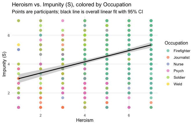

ggplot(scale_scores, aes(y = Villain_S_mean, x = Heroism, color = Cond)) +
  # points colored by condition
  geom_point(size = 2.7, alpha = 0.7) +
  # ONE lm line PER condition (because color is mapped here)
  stat_smooth(method = "lm", se = FALSE, linewidth = 1, fullrange = TRUE) +
  scale_color_brewer(palette = "Set2") +
  labs(
    y = "Impunity (S) ",
    x = "Heroism",
    color = "Occupation",
    title = "Heroism vs. Impunity (S) with per-Occupation linear fits"
  ) +
  theme_minimal(base_size = 12) +
  theme(legend.position = "right", panel.grid.minor = element_blank())

## `geom_smooth()` using formula = 'y ~ x'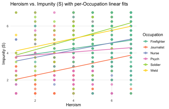

==> Full support for our hypotheses. Across all occupations Heroism predict general- and specific-level gratitude, with or without controlling for attitude.

Model 1: “~Heroism + Occupation”

# =========================
# OLD MODELS (Heroism)
# =========================
m1_H <- lm(Villain_S_mean ~ Heroism + Occupation, data = scale_scores)
m2_H <- lm(Villain_S_mean ~ Heroism * Occupation, data = scale_scores)
m3_H <- lm(Villain_S_mean ~ Heroism + Occupation + Attitude, data = scale_scores)
m4_H <- lm(Villain_S_mean ~ Heroism * Occupation + Attitude, data = scale_scores)

tidy_type3(m1_H, "~Heroism + Cond")

~Heroism + Cond
	Term	df1	df2	F	p	eta2p
Heroism	Heroism	1	833	52.23	< .001	0.059
Occupation	Occupation	5	833	34.66	< .001	0.172

# =========================
# NEW MODELS (Danger & Help)
# =========================

Model 2: “~Heroism * Occupation”

tidy_type3(m2_H, "~Heroism * Cond")

~Heroism * Cond
	Term	df1	df2	F	p	eta2p
Heroism	Heroism	1	828	45.96	< .001	0.053
Occupation	Occupation	5	828	3.94	= 0.002	0.023
Heroism:Occupation	Heroism:Occupation	5	828	1.24	= 0.290	0.007

Model 3: “~Heroism + Occupation + Attitude”

tidy_type3(m3_H, "~Heroism + Occupation + Attitude")

~Heroism + Occupation + Attitude
	Term	df1	df2	F	p	eta2p
Heroism	Heroism	1	832	2.91	= 0.088	0.003
Occupation	Occupation	5	832	34.61	< .001	0.172
Attitude	Attitude	1	832	24.42	< .001	0.029

Model 4: “~Heroism * Occupation + Attitude”

tidy_type3(m4_H, "~Heroism * Occupation + Attitude")

~Heroism * Occupation + Attitude
	Term	df1	df2	F	p	eta2p
Heroism	Heroism	1	827	3.10	= 0.079	0.004
Occupation	Occupation	5	827	2.83	= 0.015	0.017
Attitude	Attitude	1	827	21.59	< .001	0.025
Heroism:Occupation	Heroism:Occupation	5	827	0.71	= 0.616	0.004

Comparison of main predictors across models

# Use orthogonal contrasts; keeps your "Heroism main effect" interpretable with Cond in the model
old_contr <- options(contrasts = c("contr.sum", "contr.poly"))

# Helper to extract the main effect of "Heroism" from a car::Anova table
extract_heroism <- function(mod, model_label) {
  a <- car::Anova(mod, type = "III")

  # Coerce to data.frame with rownames preserved
  tab <- as.data.frame(a)
  tab$Term <- rownames(tab)

  # Standard column names across R versions
  # (car::Anova uses these names for lm/glm type=III)
  # Columns: "Sum Sq", "Df", "F value", "Pr(>F)"
  names(tab) <- sub(" ", "_", names(tab))  # make names safe: "Sum_Sq", "F_value", etc.

  # Pull rows we need
  hero <- tab %>% filter(Term == "Heroism")
  resid <- tab %>% filter(Term == "Residuals")

  # Safety checks (in case of name variants)
  stopifnot(nrow(hero) == 1, nrow(resid) == 1)

  # Partial eta^2 = SS_effect / (SS_effect + SS_residual)
  eta_p2 <- hero$Sum_Sq / (hero$Sum_Sq + resid$Sum_Sq)

  # Format p nicely (APA-ish)
  p_fmt <- ifelse(hero$`Pr(>F)` < .001, "< .001",
                  sprintf("= %.3f", hero$`Pr(>F)`))

  dplyr::tibble(
    Model = model_label,
    Outcome = "Villain_S_mean",
    Predictor = "Heroism",
    df1 = hero$Df,
    df2 = resid$Df,
    F = hero$F_value,
    p = p_fmt,
    eta2p = eta_p2
  )
}

# ----- Fit the four models -----
mod1 <- lm(Villain_S_mean ~ Heroism + Cond, data = scale_scores)
mod2 <- lm(Villain_S_mean ~ Heroism * Cond, data = scale_scores)
mod3 <- lm(Villain_S_mean ~ Heroism + Cond + scale(Attitude), data = scale_scores)
mod4 <- lm(Villain_S_mean ~ Heroism * Cond + scale(Attitude), data = scale_scores)

# ----- Build the summary table -----
tbl <- bind_rows(
  extract_heroism(mod1, "~ Heroism + Cond"),
  extract_heroism(mod2, "~ Heroism * Occupation"),
  extract_heroism(mod3, "~ Heroism + Cond + Attitude"),
  extract_heroism(mod4, "~ Heroism * Occupation + Attitude")
  ) %>%
  # Nice number formatting for F and eta^2p
  mutate(
    F = round(F, 2),
    eta2p = round(eta2p, 3)
  )

# ----- Print as HTML-friendly table -----
# Build the table first
tbl_kbl <- tbl %>%
  kable("html",
        caption = "Main effect of Heroism across models (Type-III ANOVA): F, p, partial η²",
        align = "lllrrrcr")
# Add a footnote in a version-robust way
if ("footnote" %in% getNamespaceExports("kableExtra")) {
  tbl_kbl <- tbl_kbl %>%
    kableExtra::footnote(
      general = "Type-III sums of squares with sum contrasts. Partial η² = SS_effect / (SS_effect + SS_residual). p values are APA-style.",
      general_title = ""
    )
} else {
  tbl_kbl <- tbl_kbl %>%
    kableExtra::add_footnote(
      label = "Type-III sums of squares with sum contrasts. Partial η² = SS_effect / (SS_effect + SS_residual). p values are APA-style.",
      notation = "none"
    )
}

tbl_kbl

Main effect of Heroism across models (Type-III ANOVA): F, p, partial η²
Model	Outcome	Predictor	df1	df2	F	p	eta2p
~ Heroism + Cond	Villain_S_mean	Heroism	1	833	52.23	< .001	0.059
~ Heroism * Occupation	Villain_S_mean	Heroism	1	828	45.96	< .001	0.053
~ Heroism + Cond + Attitude	Villain_S_mean	Heroism	1	832	2.91	= 0.088	0.003
~ Heroism * Occupation + Attitude	Villain_S_mean	Heroism	1	827	3.10	= 0.079	0.004
Type-III sums of squares with sum contrasts. Partial η² = SS_effect / (SS_effect + SS_residual). p values are APA-style.

Conclusion for Primary statistical models

We obtained FULL SUPPORT for H1 (Gratitude), H2 (Criticism acceptability), and H5 (Impunity). However, we obtained NO SUPPORT for H3 (support for workers demands) and H4 (victimisation). In fact, heroised occupation appeared to be supported and victimised.

Those previous analyses focus on effects of heroism across occupations. We demonstrated in previous studies that heroism was predicted by perceptions of exposure to danger and perceptions of helpfulness of the occupations. In our secondary analyses, we make the predictions that these antecedents of heroism should predict our target outcomes as well (hypothetically, through increased perceived heroism).

Secondary analyses

In a series of previous studies, we found that heroism perception can be predicted by manipulating how occupations are framed as being helpful and exposed to danger (see https://jeanmoneger.com/uploads/herofactory2025 for a full report on all studies on this topic). Because helpfulness and exposure to danger are predictors of heroism, then they should predict each target outcome through heroism. In other words, we can presume the existence of a mediation pathway whereby helpfulness and danger perception can predict heroism which in return would predict our target outcomes.

Obviously, the current study design does not enable any serious mediation analysis (see Pirlott & MacKinnon, 2016). However, we can still assess to what extent helpfulness and exposure to danger can predict the target outcomes. In particular, we can assess if these appraisals, when considered in the same model, compete against each other in predicting our outcomes. We can evaluate the relative contributions of each appraisal to each target outcomes.

In our secondary registered analyses, we planned to recycle our four models approach but replace heroism with ‘Helpulness + Danger’.

H1: Danger + Helpfulness is positively associated to gratitude

To the extent that Helpfulness and Exposure to danger are predictors of Heroism - they should also influence gratitude

General level

To what extent do you feel grateful for XXXs’ work?

Toggle details of the models diagnostics and outlier analyses

Below, you’ll find model diagnostics (QQ plot, fitted vs residuals, linearity), Outliers analysis, and more details on the output

[NOTE THAT EFFECT SIZES REPORTED IN THE REPORT COMMANDS BELOW SHOULD NOT BE TRUSTED]

paste0("####################################################")

## [1] "####################################################"

paste0("Diagnostics for Model 1: DV ~ Heroism + Occupation")

## [1] "Diagnostics for Model 1: DV ~ Heroism + Occupation"

paste0("####################################################")

## [1] "####################################################"

mod1 <- lm(Gratitude_G_mean ~ Danger+Help + Cond, data = scale_scores)
mod1r <- lmrob(Gratitude_G_mean ~ Danger+Help + Cond, data = scale_scores)

## Warning in lmrob.S(x, y, control = control): S refinements did not converge (to
## refine.tol=1e-07) in 200 (= k.max) steps

## Warning in lmrob.fit(x, y, control, init = init): initial estim. 'init' not
## converged -- will be return()ed basically unchanged

plot(mod1)

ols_plot_cooksd_bar(mod1, type = 1)

paste0("Comparison with Robust model")

## [1] "Comparison with Robust model"

models <- list("OLS (lm)" = mod1, "Robust (lmrob)" = mod1r)
modelsummary(
  models,
  statistic = c("({std.error})", "{statistic}", "p = {p.value}"),
  gof_omit  = "IC|Log.Lik",   # robust AIC comparability is iffy; omit by default
  output    = "html"
)

	OLS (lm)	Robust (lmrob)
(Intercept)	5.535	5.893
	(0.038)
	146.906
	p = <0.001
Danger	0.029	0.044
	(0.051)
	0.570
	p = 0.569
Help	1.061	1.241
	(0.052)
	20.415
	p = <0.001
Cond1	0.297	−0.045
	(0.091)
	3.252
	p = 0.001
Cond2	0.168	0.292
	(0.098)
	1.719
	p = 0.086
Cond3	0.163	−0.036
	(0.090)
	1.815
	p = 0.070
Cond4	−0.441	−0.068
	(0.090)
	−4.923
	p = <0.001
Cond5	0.030	−0.060
	(0.089)
	0.335
	p = 0.738
Num.Obs.	840	840
R2	0.514	0.953
R2 Adj.	0.509	0.952
RMSE	1.09	1.17

fitted_vals <- fitted(mod1)

# Plot observed values against fitted values
plot(fitted_vals, scale_scores$Gratitude_G_mean,
     xlab = "Fitted Values",
     ylab = "Observed DV",
     main = "Observed vs Fitted Values")
abline(0, 1, col = "blue", lty = 2)

paste0("####################################################")

## [1] "####################################################"

paste0("Diagnostics for Model 2: DV ~ Heroism * Occupation")

## [1] "Diagnostics for Model 2: DV ~ Heroism * Occupation"

paste0("####################################################")

## [1] "####################################################"

mod1 <- lm(Gratitude_G_mean ~ Danger + Help +Danger:Cond + Help:Cond, data = scale_scores)
mod1r <- lmrob(Gratitude_G_mean ~ Danger + Help +Danger:Cond + Help:Cond, data = scale_scores)

## Warning in lmrob.S(x, y, control = control): S refinements did not converge (to
## refine.tol=1e-07) in 200 (= k.max) steps
## Warning in lmrob.S(x, y, control = control): initial estim. 'init' not
## converged -- will be return()ed basically unchanged

plot(mod1)

ols_plot_cooksd_bar(mod1, type = 1)

paste0("Comparison with Robust model")

## [1] "Comparison with Robust model"

models <- list("OLS (lm)" = mod1, "Robust (lmrob)" = mod1r)
modelsummary(
  models,
  statistic = c("({std.error})", "{statistic}", "p = {p.value}"),
  gof_omit  = "IC|Log.Lik",   # robust AIC comparability is iffy; omit by default
  output    = "html"
)

	OLS (lm)	Robust (lmrob)
(Intercept)	5.470	5.818
	(0.051)
	107.199
	p = <0.001
Danger	0.142	0.198
	(0.069)
	2.067
	p = 0.039
Help	0.987	1.089
	(0.071)
	13.940
	p = <0.001
Danger × Cond1	0.479	−0.158
	(0.276)
	1.736
	p = 0.083
Danger × Cond2	−0.122	0.566
	(0.110)
	−1.111
	p = 0.267
Danger × Cond3	−0.028	−0.166
	(0.110)
	−0.255
	p = 0.799
Danger × Cond4	0.013	−0.185
	(0.101)
	0.125
	p = 0.901
Danger × Cond5	−0.120	−0.164
	(0.121)
	−0.991
	p = 0.322
Help × Cond1	−0.123	0.188
	(0.292)
	−0.421
	p = 0.674
Help × Cond2	−0.020	−0.643
	(0.107)
	−0.188
	p = 0.851
Help × Cond3	0.406	0.221
	(0.125)
	3.244
	p = 0.001
Help × Cond4	−0.321	0.186
	(0.121)
	−2.641
	p = 0.008
Help × Cond5	0.286	0.199
	(0.102)
	2.808
	p = 0.005
Num.Obs.	840	840
R2	0.519	0.963
R2 Adj.	0.512	0.962
RMSE	1.08	1.20

fitted_vals <- fitted(mod1)

# Plot observed values against fitted values
plot(fitted_vals, scale_scores$Gratitude_G_mean,
     xlab = "Fitted Values",
     ylab = "Observed DV",
     main = "Observed vs Fitted Values")
abline(0, 1, col = "blue", lty = 2)

paste0("####################################################")

## [1] "####################################################"

paste0("Diagnostics for Model 3: DV ~ Heroism + Occupation + Attitude")

## [1] "Diagnostics for Model 3: DV ~ Heroism + Occupation + Attitude"

paste0("####################################################")

## [1] "####################################################"

mod1 <- lm(Gratitude_G_mean ~ Danger + Help + Occupation + Attitude, data = scale_scores)
mod1r <- lmrob(Gratitude_G_mean ~ Danger + Help + Occupation + Attitude, data = scale_scores)

## Warning in lmrob.S(x, y, control = control): find_scale() did not converge in
## 'maxit.scale' (= 200) iterations with tol=1e-10, last rel.diff=0

## Warning in lmrob.S(x, y, control = control): S-estimated scale == 0: Probably
## exact fit; check your data

## Warning in lmrob.fit(x, y, control, init = init): initial estim. 'init' not
## converged -- will be return()ed basically unchanged

plot(mod1)

ols_plot_cooksd_bar(mod1, type = 1)

paste0("Comparison with Robust model")

## [1] "Comparison with Robust model"

models <- list("OLS (lm)" = mod1, "Robust (lmrob)" = mod1r)
modelsummary(
  models,
  statistic = c("({std.error})", "{statistic}", "p = {p.value}"),
  gof_omit  = "IC|Log.Lik",   # robust AIC comparability is iffy; omit by default
  output    = "html"
)

	OLS (lm)	Robust (lmrob)
(Intercept)	5.535	5.506
	(0.031)	(0.000)
	178.264
	p = <0.001
Danger	−0.032	0.000
	(0.042)	(0.000)
	−0.762
	p = 0.446
Help	0.310	0.000
	(0.057)	(0.000)
	5.415
	p = <0.001
Occupation1	0.179	0.167
	(0.075)	(0.000)
	2.369
	p = 0.018
Occupation2	0.260	0.167
	(0.081)	(0.000)
	3.217
	p = 0.001
Occupation3	0.064	0.167
	(0.074)	(0.000)
	0.867
	p = 0.386
Occupation4	−0.296	0.167
	(0.074)	(0.000)
	−3.980
	p = <0.001
Occupation5	0.012	0.167
	(0.073)	(0.000)
	0.168
	p = 0.867
Attitude	1.030	1.291
	(0.052)	(0.000)
	19.850
	p = <0.001
Num.Obs.	840	840
R2	0.670	1.000
R2 Adj.	0.667	1.000
RMSE	0.90	0.96

fitted_vals <- fitted(mod1)

# Plot observed values against fitted values
plot(fitted_vals, scale_scores$Gratitude_G_mean,
     xlab = "Fitted Values",
     ylab = "Observed DV",
     main = "Observed vs Fitted Values")
abline(0, 1, col = "blue", lty = 2)

paste0("####################################################")

## [1] "####################################################"

paste0("Diagnostics for Model 4: DV ~ Heroism * Occupation + Attitude")

## [1] "Diagnostics for Model 4: DV ~ Heroism * Occupation + Attitude"

paste0("####################################################")

## [1] "####################################################"

mod1 <- lm(Gratitude_G_mean ~ Danger + Help + Occupation + Danger:Occupation + Help:Occupation + Attitude, data = scale_scores)
mod1r <- lmrob(Villain_S_mean ~ Danger + Help + Occupation + Danger:Occupation + Help:Occupation + Attitude, data = scale_scores)
plot(mod1)

ols_plot_cooksd_bar(mod1, type = 1)

paste0("Comparison with Robust model")

## [1] "Comparison with Robust model"

models <- list("OLS (lm)" = mod1, "Robust (lmrob)" = mod1r)
modelsummary(
  models,
  statistic = c("({std.error})", "{statistic}", "p = {p.value}"),
  gof_omit  = "IC|Log.Lik",   # robust AIC comparability is iffy; omit by default
  output    = "html"
)

	OLS (lm)	Robust (lmrob)
(Intercept)	5.536	4.612
	(0.044)	(0.075)
	125.031	61.610
	p = <0.001	p = <0.001
Danger	−0.041	0.122
	(0.061)	(0.098)
	−0.664	1.236
	p = 0.507	p = 0.217
Help	0.335	0.114
	(0.072)	(0.111)
	4.675	1.029
	p = <0.001	p = 0.304
Occupation1	0.092	−0.273
	(0.125)	(0.162)
	0.737	−1.685
	p = 0.461	p = 0.092
Occupation2	0.269	−1.493
	(0.100)	(0.180)
	2.695	−8.310
	p = 0.007	p = <0.001
Occupation3	0.041	0.248
	(0.101)	(0.205)
	0.407	1.210
	p = 0.684	p = 0.227
Occupation4	−0.279	−0.331
	(0.087)	(0.186)
	−3.207	−1.783
	p = 0.001	p = 0.075
Occupation5	0.088	0.947
	(0.089)	(0.125)
	0.992	7.567
	p = 0.321	p = <0.001
Attitude	1.002	0.454
	(0.053)	(0.104)
	18.895	4.356
	p = <0.001	p = <0.001
Danger × Occupation1	0.005	−0.288
	(0.239)	(0.317)
	0.022	−0.907
	p = 0.982	p = 0.365
Danger × Occupation2	0.058	−0.302
	(0.094)	(0.167)
	0.624	−1.806
	p = 0.533	p = 0.071
Danger × Occupation3	0.079	0.560
	(0.097)	(0.180)
	0.814	3.114
	p = 0.416	p = 0.002
Danger × Occupation4	0.015	0.069
	(0.090)	(0.161)
	0.168	0.429
	p = 0.867	p = 0.668
Danger × Occupation5	−0.103	0.135
	(0.114)	(0.175)
	−0.907	0.772
	p = 0.365	p = 0.440
Help × Occupation1	0.134	0.301
	(0.248)	(0.326)
	0.539	0.923
	p = 0.590	p = 0.356
Help × Occupation2	−0.029	−0.021
	(0.097)	(0.171)
	−0.294	−0.124
	p = 0.769	p = 0.902
Help × Occupation3	0.058	−0.425
	(0.131)	(0.251)
	0.445	−1.694
	p = 0.657	p = 0.091
Help × Occupation4	−0.148	−0.136
	(0.107)	(0.212)
	−1.392	−0.643
	p = 0.164	p = 0.521
Help × Occupation5	0.136	0.072
	(0.089)	(0.147)
	1.530	0.493
	p = 0.126	p = 0.622
Num.Obs.	840	840
R2	0.675	0.343
R2 Adj.	0.668	0.329
RMSE	0.89	1.55

fitted_vals <- fitted(mod1)

# Plot observed values against fitted values
plot(fitted_vals, scale_scores$Gratitude_G_mean,
     xlab = "Fitted Values",
     ylab = "Observed DV",
     main = "Observed vs Fitted Values")
abline(0, 1, col = "blue", lty = 2)

paste0("####################################################")

## [1] "####################################################"

paste0("REPORTS for each model (please ignore the eta squares, they are way off")

## [1] "REPORTS for each model (please ignore the eta squares, they are way off"

paste0("####################################################")

## [1] "####################################################"

paste0("MODEL 1: Gratitude_G_mean ~ Danger+Helpfulness")

## [1] "MODEL 1: Gratitude_G_mean ~ Danger+Helpfulness"

report(Anova(mod1 <- lm(Gratitude_G_mean ~ Danger+Help + Cond, data = scale_scores), type = "III"))

## The ANOVA suggests that:
## 
##   - The main effect of Danger is statistically not significant and very small
## (F(1, 832) = 0.32, p = 0.569; Eta2 (partial) = 3.90e-04, 95% CI [0.00, 1.00])
##   - The main effect of Help is statistically significant and large (F(1, 832) =
## 416.77, p < .001; Eta2 (partial) = 0.33, 95% CI [0.29, 1.00])
##   - The main effect of Cond is statistically significant and small (F(5, 832) =
## 8.85, p < .001; Eta2 (partial) = 0.05, 95% CI [0.03, 1.00])
## 
## Effect sizes were labelled following Field's (2013) recommendations.

paste0("MODEL 2: Gratitude_G_mean ~ Danger+Help * Cond")

## [1] "MODEL 2: Gratitude_G_mean ~ Danger+Help * Cond"

report(Anova(mod2 <- lm(Gratitude_G_mean ~ Danger + Help +Danger:Cond + Help:Cond, data = scale_scores), type = "III"))

## Type 3 ANOVAs only give sensible and informative results when covariates
##   are mean-centered and factors are coded with orthogonal contrasts (such
##   as those produced by `contr.sum`, `contr.poly`, or `contr.helmert`, but
##   *not* by the default `contr.treatment`).

## The ANOVA suggests that:
## 
##   - The main effect of Danger is statistically significant and very small (F(1,
## 827) = 4.27, p = 0.039; Eta2 (partial) = 5.14e-03, 95% CI [1.35e-04, 1.00])
##   - The main effect of Help is statistically significant and large (F(1, 827) =
## 194.33, p < .001; Eta2 (partial) = 0.19, 95% CI [0.15, 1.00])
##   - The interaction between Danger and Cond is statistically not significant and
## very small (F(5, 827) = 1.07, p = 0.376; Eta2 (partial) = 6.42e-03, 95% CI
## [0.00, 1.00])
##   - The interaction between Help and Cond is statistically significant and small
## (F(5, 827) = 6.31, p < .001; Eta2 (partial) = 0.04, 95% CI [0.01, 1.00])
## 
## Effect sizes were labelled following Field's (2013) recommendations.

report(Anova(mod2 <- lm(Gratitude_G_mean ~ Danger + Help + Cond + Danger:Cond + Help:Cond, data = scale_scores), type = "III"))

## Type 3 ANOVAs only give sensible and informative results when covariates
##   are mean-centered and factors are coded with orthogonal contrasts (such
##   as those produced by `contr.sum`, `contr.poly`, or `contr.helmert`, but
##   *not* by the default `contr.treatment`).

## The ANOVA suggests that:
## 
##   - The main effect of Danger is statistically not significant and very small
## (F(1, 822) = 1.89, p = 0.169; Eta2 (partial) = 2.30e-03, 95% CI [0.00, 1.00])
##   - The main effect of Help is statistically significant and large (F(1, 822) =
## 170.54, p < .001; Eta2 (partial) = 0.17, 95% CI [0.14, 1.00])
##   - The main effect of Cond is statistically significant and small (F(5, 822) =
## 5.20, p < .001; Eta2 (partial) = 0.03, 95% CI [0.01, 1.00])
##   - The interaction between Danger and Cond is statistically not significant and
## very small (F(5, 822) = 0.96, p = 0.442; Eta2 (partial) = 5.80e-03, 95% CI
## [0.00, 1.00])
##   - The interaction between Help and Cond is statistically significant and small
## (F(5, 822) = 4.77, p < .001; Eta2 (partial) = 0.03, 95% CI [8.64e-03, 1.00])
## 
## Effect sizes were labelled following Field's (2013) recommendations.

paste0("MODEL 3: Gratitude_G_mean ~ Danger+Help +scale(Attitude)")

## [1] "MODEL 3: Gratitude_G_mean ~ Danger+Help +scale(Attitude)"

report(Anova(mod3 <- lm(Gratitude_G_mean ~Danger + Help + Occupation + Attitude , data = scale_scores), type = "III"))

## The ANOVA suggests that:
## 
##   - The main effect of Danger is statistically not significant and very small
## (F(1, 831) = 0.58, p = 0.446; Eta2 (partial) = 6.98e-04, 95% CI [0.00, 1.00])
##   - The main effect of Help is statistically significant and small (F(1, 831) =
## 29.33, p < .001; Eta2 (partial) = 0.03, 95% CI [0.02, 1.00])
##   - The main effect of Occupation is statistically significant and small (F(5,
## 831) = 8.08, p < .001; Eta2 (partial) = 0.05, 95% CI [0.02, 1.00])
##   - The main effect of Attitude is statistically significant and large (F(1, 831)
## = 394.03, p < .001; Eta2 (partial) = 0.32, 95% CI [0.28, 1.00])
## 
## Effect sizes were labelled following Field's (2013) recommendations.

paste0("MODEL 4: Gratitude_G_mean ~ Danger+Help * Cond + scale(Attitude)")

## [1] "MODEL 4: Gratitude_G_mean ~ Danger+Help * Cond + scale(Attitude)"

report(Anova(mod4 <-lm(Gratitude_G_mean ~ Danger + Help + Cond + Danger:Cond + Help:Cond + scale(Attitude), data = scale_scores), type = "III"))

## Type 3 ANOVAs only give sensible and informative results when covariates
##   are mean-centered and factors are coded with orthogonal contrasts (such
##   as those produced by `contr.sum`, `contr.poly`, or `contr.helmert`, but
##   *not* by the default `contr.treatment`).

## The ANOVA suggests that:
## 
##   - The main effect of Danger is statistically not significant and very small
## (F(1, 821) = 0.44, p = 0.507; Eta2 (partial) = 5.36e-04, 95% CI [0.00, 1.00])
##   - The main effect of Help is statistically significant and small (F(1, 821) =
## 21.85, p < .001; Eta2 (partial) = 0.03, 95% CI [0.01, 1.00])
##   - The main effect of Cond is statistically significant and small (F(5, 821) =
## 4.30, p < .001; Eta2 (partial) = 0.03, 95% CI [6.84e-03, 1.00])
##   - The main effect of scale(Attitude) is statistically significant and large
## (F(1, 821) = 357.02, p < .001; Eta2 (partial) = 0.30, 95% CI [0.26, 1.00])
##   - The interaction between Danger and Cond is statistically not significant and
## very small (F(5, 821) = 0.40, p = 0.847; Eta2 (partial) = 2.45e-03, 95% CI
## [0.00, 1.00])
##   - The interaction between Help and Cond is statistically not significant and
## very small (F(5, 821) = 1.48, p = 0.195; Eta2 (partial) = 8.90e-03, 95% CI
## [0.00, 1.00])
## 
## Effect sizes were labelled following Field's (2013) recommendations.

paste0("Model Comparison: assessing the importance of attitude - not accounting for occupations")

## [1] "Model Comparison: assessing the importance of attitude - not accounting for occupations"

anova(mod1, mod3)

paste0("Model Comparison: assessing the importance of attitude - accounting for occupations")

## [1] "Model Comparison: assessing the importance of attitude - accounting for occupations"

anova(mod2, mod4)

# Build long data for faceting (DV = Gratitude_G_mean)
plot_df <- scale_scores %>%
  dplyr::select(Gratitude_G_mean, Danger, Help, Cond) %>%
  dplyr::filter(!is.na(Gratitude_G_mean), !is.na(Danger), !is.na(Help)) %>%
  dplyr::mutate(Cond = as.factor(Cond)) %>%
  tidyr::pivot_longer(
    cols = c(Danger, Help),
    names_to = "Predictor",
    values_to = "X"
  )

## Warning: Using one column matrices in `filter()` was deprecated in dplyr 1.1.0.
## ℹ Please use one dimensional logical vectors instead.
## This warning is displayed once every 8 hours.
## Call `lifecycle::last_lifecycle_warnings()` to see where this warning was
## generated.

# ------------- Version 1: ONE global lm line per facet + 95% CI -------------
p_global <- ggplot2::ggplot(plot_df, ggplot2::aes(x = X, y = Gratitude_G_mean)) +
  ggplot2::geom_point(ggplot2::aes(color = Cond), alpha = 0.7, size = 2.6) +
  ggplot2::stat_smooth(
    method = "lm", se = TRUE, level = 0.95,
    ggplot2::aes(group = 1),
    color = "black", fill = "grey60", alpha = 0.20, linewidth = 1
  ) +
  ggplot2::facet_wrap(
    ~ Predictor, ncol = 2,
    labeller = ggplot2::as_labeller(c(Danger = "Danger → Gratitude",
                                      Help   = "Help → Gratitude"))
    # , scales = "free_x"
  ) +
  ggplot2::scale_color_brewer(palette = "Set2") +
  ggplot2::labs(
    x = "Predictor value", y = "Gratitude (G) — Mean",
    color = "Condition",
    title = "Gratitude vs Danger/Help (global fit per facet)",
    subtitle = "Black line = overall linear fit; shaded band = 95% CI"
  ) +
  ggplot2::theme_minimal(base_size = 12) +
  ggplot2::theme(panel.grid.minor = ggplot2::element_blank(),
                 strip.text = ggplot2::element_text(face = "bold"))

# ------------- Version 2: PER-Cond lm lines + 95% CI -------------
p_by_cond <- ggplot2::ggplot(plot_df, ggplot2::aes(x = X, y = Gratitude_G_mean, color = Cond)) +
  ggplot2::geom_point(alpha = 0.7, size = 2.6) +
  ggplot2::stat_smooth(
    method = "lm", se = TRUE, level = 0.95,
    ggplot2::aes(fill = Cond),  # ribbons match line colors
    alpha = 0.15, linewidth = 1
  ) +
  ggplot2::facet_wrap(
    ~ Predictor, ncol = 2,
    labeller = ggplot2::as_labeller(c(Danger = "Danger → Gratitude",
                                      Help   = "Help → Gratitude"))
    # , scales = "free_x"
  ) +
  ggplot2::scale_color_brewer(palette = "Set2") +
  ggplot2::scale_fill_brewer(palette = "Set2", guide = "none") + # avoid duplicate legend
  ggplot2::labs(
    x = "Predictor value", y = "Gratitude (G) — Mean",
    color = "Condition",
    title = "Gratitude vs Danger/Help (separate fits per Cond)",
    subtitle = "One linear fit per condition; shaded bands = 95% CI"
  ) +
  ggplot2::theme_minimal(base_size = 12) +
  ggplot2::theme(panel.grid.minor = ggplot2::element_blank(),
                 strip.text = ggplot2::element_text(face = "bold"))

p_global

## `geom_smooth()` using formula = 'y ~ x'

p_by_cond

## `geom_smooth()` using formula = 'y ~ x'

Model 1: “~Heroism + Occupation”

m1_DH <- lm(Gratitude_G_mean ~ Danger + Help + Occupation, data = scale_scores)
m2_DH <- lm(Gratitude_G_mean ~ Danger + Help + Occupation + Danger:Occupation + Help:Occupation, data = scale_scores)
m3_DH <- lm(Gratitude_G_mean ~ Danger + Help + Occupation + Attitude, data = scale_scores)
m4_DH <- lm(Gratitude_G_mean ~ Danger + Help + Occupation + Danger:Occupation + Help:Occupation + Attitude, data = scale_scores)

tidy_type3(m1_DH, "~ Danger + Help + Cond")

~ Danger + Help + Cond
	Term	df1	df2	F	p	eta2p
Danger	Danger	1	832	0.32	= 0.569	0.000
Help	Help	1	832	416.77	< .001	0.334
Occupation	Occupation	5	832	8.85	< .001	0.051

#
#
#

Model 2: “~ Danger + Help + Danger:Cond + Help:Cond”

tidy_type3(m2_DH, "~ Danger + Help + Danger:Cond + Help:Cond")

~ Danger + Help + Danger:Cond + Help:Cond
	Term	df1	df2	F	p	eta2p
Danger	Danger	1	822	1.89	= 0.169	0.002
Help	Help	1	822	170.54	< .001	0.172
Occupation	Occupation	5	822	5.20	< .001	0.031
Danger:Occupation	Danger:Occupation	5	822	0.96	= 0.442	0.006
Help:Occupation	Help:Occupation	5	822	4.77	< .001	0.028

Model 3: “~Danger + Help + Occupation + Attitude”

tidy_type3(m3_DH, "~ Danger + Help + Cond + scale(Attitude)")

~ Danger + Help + Cond + scale(Attitude)
	Term	df1	df2	F	p	eta2p
Danger	Danger	1	831	0.58	= 0.446	0.001
Help	Help	1	831	29.33	< .001	0.034
Occupation	Occupation	5	831	8.08	< .001	0.046
Attitude	Attitude	1	831	394.03	< .001	0.322

Model 4: “~Danger + Help + Danger:Cond + Help:Cond + Attitude”

tidy_type3(m4_DH, "~ Danger + Help + Cond + Danger:Cond + Help:Cond + Attitude")

~ Danger + Help + Cond + Danger:Cond + Help:Cond + Attitude
	Term	df1	df2	F	p	eta2p
Danger	Danger	1	821	0.44	= 0.507	0.001
Help	Help	1	821	21.85	< .001	0.026
Occupation	Occupation	5	821	4.30	< .001	0.025
Attitude	Attitude	1	821	357.02	< .001	0.303
Danger:Occupation	Danger:Occupation	5	821	0.40	= 0.847	0.002
Help:Occupation	Help:Occupation	5	821	1.48	= 0.195	0.009

Comparison of main predictors across models

old_contr <- options(contrasts = c("contr.sum", "contr.poly"))

# =========================
# Ensure factor names exist and are factors
# - If your data already has 'Occupation', this keeps it.
# - If not, but you have 'Cond', we'll mirror it to 'Occupation'.
# =========================
if (!"Occupation" %in% names(scale_scores) && "Cond" %in% names(scale_scores)) {
  scale_scores <- scale_scores %>% mutate(Occupation = Cond)
}
scale_scores <- scale_scores %>% mutate(Occupation = as.factor(Occupation))

# =========================
# Helper: partial eta^2 from F and dfs (matches effectsize)
# η²p = (F * df1) / (F * df1 + df2)
# =========================
eta_p2_fromF <- function(Fval, df1, df2) (Fval * df1) / (Fval * df1 + df2)

# =========================
# Pull stats for a given term from a Type-III ANOVA
# Returns: df1, df2, F (rounded), p (APA-ish), eta2p (rounded)
# =========================
pull_term <- function(mod, term_name) {
  a <- car::Anova(mod, type = "III")
  tab <- as.data.frame(a)
  tab$Term <- rownames(tab)
  names(tab) <- sub(" ", "_", names(tab))  # "Sum Sq" -> "Sum_Sq", "F value" -> "F_value", etc.

  row_term  <- dplyr::filter(tab, Term == term_name)
  row_resid <- dplyr::filter(tab, Term == "Residuals")
  stopifnot(nrow(row_term) == 1, nrow(row_resid) == 1)

  df1 <- row_term$Df
  df2 <- row_resid$Df
  Fv  <- row_term$F_value
  pv  <- row_term$`Pr(>F)`

  tibble(
    df1   = df1,
    df2   = df2,
    F     = round(Fv, 2),
    p     = ifelse(pv < .001, "< .001", sprintf("= %.3f", pv)),
    eta2p = round(eta_p2_fromF(Fv, df1, df2), 3)
  )
}

# =========================
# Fit the four models (as specified)
# NOTE: If your variable is 'Helpfulness' instead of 'Help', replace 'Help' below.
# =========================
m1_DH <- lm(Gratitude_G_mean ~ Danger + Help + Occupation, data = scale_scores)
m2_DH <- lm(Gratitude_G_mean ~ Danger + Help + Occupation + Danger:Occupation + Help:Occupation, data = scale_scores)
m3_DH <- lm(Gratitude_G_mean ~ Danger + Help + Occupation + Attitude, data = scale_scores)
m4_DH <- lm(Gratitude_G_mean ~ Danger + Help + Occupation + Danger:Occupation + Help:Occupation + Attitude, data = scale_scores)

# =========================
# One row per model, with Danger_* and Help_* side-by-side
# =========================
row_for_model <- function(mod, label) {
  d_stats <- pull_term(mod, "Danger") %>% rename_with(~ paste0("Danger_", .x))
  h_stats <- pull_term(mod, "Help")   %>% rename_with(~ paste0("Help_",   .x))
  tibble(Model = label, Outcome = "Gratitude G") %>%
    bind_cols(d_stats, h_stats)
}

comp_tbl <- bind_rows(
  row_for_model(m1_DH, "~ Danger + Help + Occupation"),
  row_for_model(m2_DH, "~ Danger + Help + Occupation + Danger:Occupation + Help:Occupation"),
  row_for_model(m3_DH, "~ Danger + Help + Occupation + Attitude"),
  row_for_model(m4_DH, "~ Danger + Help + Occupation + Danger:Occupation + Help:Occupation + Attitude")
)

# =========================
# Base HTML table (works without kableExtra)
# =========================
align_vec <- c("l","l", "r","r","r","c","r", "r","r","r","c","r")
kbl <- knitr::kable(
  comp_tbl,
  format  = "html",
  align   = align_vec,
  caption = "Main effects of Danger and Help across models (Type-III ANOVA). Partial η² = (F·df1) / (F·df1 + df2)."
)

# =========================
# Strong visual separation between Danger and Help (if kableExtra is installed)
# - Group headers
# - Thick vertical divider between blocks
# - Light tint on Help block
# =========================
if (isTRUE(requireNamespace("kableExtra", quietly = TRUE))) {
  danger_cols <- which(startsWith(names(comp_tbl), "Danger_"))
  help_cols   <- which(startsWith(names(comp_tbl),   "Help_"))
  idx_last_danger <- max(danger_cols)
  idx_first_help  <- min(help_cols)

  kbl <- kbl %>%
    kableExtra::kable_styling(full_width = FALSE, bootstrap_options = c("striped","hover")) %>%
    kableExtra::add_header_above(
      c(" " = 2, "Danger main effect" = length(danger_cols), "Help main effect" = length(help_cols))
    ) %>%
    # Strong divider between blocks
    kableExtra::column_spec(idx_last_danger, border_right = "3px solid #333",
                            extra_css = "padding-right:12px;") %>%
    kableExtra::column_spec(idx_first_help,  border_left  = "3px solid #333",
                            extra_css = "padding-left:12px;") %>%
    # Optional: light tint on the Help block
    # Optional: micro separators inside each block (p vs eta2p)
    kableExtra::column_spec(danger_cols[4], border_right = "1px solid #ddd",
                            extra_css = "padding-right:10px;") %>% # Danger_p
    kableExtra::column_spec(danger_cols[5], extra_css = "padding-left:10px;") %>% # Danger_eta2p
    kableExtra::column_spec(help_cols[4],   border_right = "1px solid #ddd",
                            extra_css = "padding-right:10px;") %>% # Help_p
    kableExtra::column_spec(help_cols[5],   extra_css = "padding-left:10px;")      # Help_eta2p
}

kbl

Main effects of Danger and Help across models (Type-III ANOVA). Partial η² = (F·df1) / (F·df1 + df2).
		Danger main effect					Help main effect
Model	Outcome	Danger_df1	Danger_df2	Danger_F	Danger_p	Danger_eta2p	Help_df1	Help_df2	Help_F	Help_p	Help_eta2p
~ Danger + Help + Occupation	Gratitude G	1	832	0.32	= 0.569	0.000	1	832	416.77	< .001	0.334
~ Danger + Help + Occupation + Danger:Occupation + Help:Occupation	Gratitude G	1	822	1.89	= 0.169	0.002	1	822	170.54	< .001	0.172
~ Danger + Help + Occupation + Attitude	Gratitude G	1	831	0.58	= 0.446	0.001	1	831	29.33	< .001	0.034
~ Danger + Help + Occupation + Danger:Occupation + Help:Occupation + Attitude	Gratitude G	1	821	0.44	= 0.507	0.001	1	821	21.85	< .001	0.026

Specific level

[If there were a public campaign in support of journalists, how likely would you be to do each of these things in response?] Sharing a supportive post about journalists on my social media

Toggle details of the models diagnostics and outlier analyses

Below, you’ll find model diagnostics (QQ plot, fitted vs residuals, linearity), Outliers analysis, and more details on the output

[NOTE THAT EFFECT SIZES REPORTED IN THE REPORT COMMANDS BELOW SHOULD NOT BE TRUSTED]

paste0("####################################################")

## [1] "####################################################"

paste0("Diagnostics for Model 1: DV ~ Heroism + Occupation")

## [1] "Diagnostics for Model 1: DV ~ Heroism + Occupation"

paste0("####################################################")

## [1] "####################################################"

mod1 <- lm(Gratitude_S_mean ~ Danger+Help + Cond, data = scale_scores)
mod1r <- lmrob(Gratitude_S_mean ~ Danger+Help + Cond, data = scale_scores)
plot(mod1)

ols_plot_cooksd_bar(mod1, type = 1)

paste0("Comparison with Robust model")

## [1] "Comparison with Robust model"

models <- list("OLS (lm)" = mod1, "Robust (lmrob)" = mod1r)
modelsummary(
  models,
  statistic = c("({std.error})", "{statistic}", "p = {p.value}"),
  gof_omit  = "IC|Log.Lik",   # robust AIC comparability is iffy; omit by default
  output    = "html"
)

	OLS (lm)	Robust (lmrob)
(Intercept)	3.297	3.285
	(0.055)	(0.059)
	60.288	55.488
	p = <0.001	p = <0.001
Danger	0.069	0.068
	(0.074)	(0.077)
	0.943	0.882
	p = 0.346	p = 0.378
Help	0.569	0.599
	(0.075)	(0.074)
	7.540	8.098
	p = <0.001	p = <0.001
Cond1	0.105	0.135
	(0.132)	(0.151)
	0.794	0.892
	p = 0.427	p = 0.373
Cond2	−0.216	−0.227
	(0.142)	(0.150)
	−1.523	−1.516
	p = 0.128	p = 0.130
Cond3	0.387	0.419
	(0.130)	(0.140)
	2.965	2.985
	p = 0.003	p = 0.003
Cond4	−0.257	−0.313
	(0.130)	(0.154)
	−1.978	−2.030
	p = 0.048	p = 0.043
Cond5	0.086	0.084
	(0.129)	(0.141)
	0.663	0.594
	p = 0.508	p = 0.553
Num.Obs.	840	840
R2	0.171	0.177
R2 Adj.	0.164	0.170
RMSE	1.58	1.58

fitted_vals <- fitted(mod1)

# Plot observed values against fitted values
plot(fitted_vals, scale_scores$Gratitude_S_mean,
     xlab = "Fitted Values",
     ylab = "Observed DV",
     main = "Observed vs Fitted Values")
abline(0, 1, col = "blue", lty = 2)

paste0("####################################################")

## [1] "####################################################"

paste0("Diagnostics for Model 2: DV ~ Heroism * Occupation")

## [1] "Diagnostics for Model 2: DV ~ Heroism * Occupation"

paste0("####################################################")

## [1] "####################################################"

mod1 <- lm(Gratitude_S_mean ~ Danger + Help +Danger:Cond + Help:Cond, data = scale_scores)
mod1r <- lmrob(Gratitude_S_mean ~ Danger + Help +Danger:Cond + Help:Cond, data = scale_scores)
plot(mod1)

ols_plot_cooksd_bar(mod1, type = 1)

paste0("Comparison with Robust model")

## [1] "Comparison with Robust model"

models <- list("OLS (lm)" = mod1, "Robust (lmrob)" = mod1r)
modelsummary(
  models,
  statistic = c("({std.error})", "{statistic}", "p = {p.value}"),
  gof_omit  = "IC|Log.Lik",   # robust AIC comparability is iffy; omit by default
  output    = "html"
)

	OLS (lm)	Robust (lmrob)
(Intercept)	3.355	3.334
	(0.074)	(0.086)
	45.630	38.574
	p = <0.001	p = <0.001
Danger	0.270	0.300
	(0.099)	(0.093)
	2.726	3.237
	p = 0.007	p = 0.001
Help	0.377	0.378
	(0.102)	(0.091)
	3.691	4.165
	p = <0.001	p = <0.001
Danger × Cond1	1.099	1.199
	(0.398)	(0.341)
	2.762	3.519
	p = 0.006	p = <0.001
Danger × Cond2	−0.176	−0.185
	(0.158)	(0.142)
	−1.112	−1.304
	p = 0.267	p = 0.193
Danger × Cond3	−0.075	−0.120
	(0.158)	(0.180)
	−0.473	−0.666
	p = 0.636	p = 0.506
Danger × Cond4	−0.039	−0.045
	(0.146)	(0.171)
	−0.265	−0.264
	p = 0.791	p = 0.792
Danger × Cond5	−0.265	−0.249
	(0.174)	(0.182)
	−1.527	−1.369
	p = 0.127	p = 0.172
Help × Cond1	−1.204	−1.284
	(0.421)	(0.343)
	−2.862	−3.748
	p = 0.004	p = <0.001
Help × Cond2	0.318	0.310
	(0.155)	(0.123)
	2.053	2.531
	p = 0.040	p = 0.012
Help × Cond3	0.538	0.628
	(0.181)	(0.199)
	2.979	3.161
	p = 0.003	p = 0.002
Help × Cond4	−0.316	−0.323
	(0.175)	(0.222)
	−1.804	−1.452
	p = 0.072	p = 0.147
Help × Cond5	0.537	0.539
	(0.147)	(0.118)
	3.665	4.557
	p = <0.001	p = <0.001
Num.Obs.	840	840
R2	0.191	0.193
R2 Adj.	0.180	0.181
RMSE	1.56	1.56

fitted_vals <- fitted(mod1)

# Plot observed values against fitted values
plot(fitted_vals, scale_scores$Gratitude_S_mean,
     xlab = "Fitted Values",
     ylab = "Observed DV",
     main = "Observed vs Fitted Values")
abline(0, 1, col = "blue", lty = 2)

paste0("####################################################")

## [1] "####################################################"

paste0("Diagnostics for Model 3: DV ~ Heroism + Occupation + Attitude")

## [1] "Diagnostics for Model 3: DV ~ Heroism + Occupation + Attitude"

paste0("####################################################")

## [1] "####################################################"

mod1 <- lm(Gratitude_S_mean ~ Danger + Help + Occupation + Attitude, data = scale_scores)
mod1r <- lmrob(Gratitude_S_mean ~ Danger + Help + Occupation + Attitude, data = scale_scores)
plot(mod1)

ols_plot_cooksd_bar(mod1, type = 1)

paste0("Comparison with Robust model")

## [1] "Comparison with Robust model"

models <- list("OLS (lm)" = mod1, "Robust (lmrob)" = mod1r)
modelsummary(
  models,
  statistic = c("({std.error})", "{statistic}", "p = {p.value}"),
  gof_omit  = "IC|Log.Lik",   # robust AIC comparability is iffy; omit by default
  output    = "html"
)

	OLS (lm)	Robust (lmrob)
(Intercept)	3.297	3.300
	(0.051)	(0.055)
	64.517	60.073
	p = <0.001	p = <0.001
Danger	0.014	−0.003
	(0.069)	(0.073)
	0.200	−0.047
	p = 0.842	p = 0.962
Help	−0.119	−0.145
	(0.094)	(0.090)
	−1.261	−1.615
	p = 0.207	p = 0.107
Occupation1	−0.003	0.009
	(0.124)	(0.142)
	−0.023	0.063
	p = 0.982	p = 0.950
Occupation2	−0.132	−0.155
	(0.133)	(0.137)
	−0.997	−1.131
	p = 0.319	p = 0.258
Occupation3	0.296	0.329
	(0.122)	(0.129)
	2.426	2.548
	p = 0.015	p = 0.011
Occupation4	−0.124	−0.149
	(0.122)	(0.134)
	−1.015	−1.109
	p = 0.311	p = 0.268
Occupation5	0.070	0.084
	(0.121)	(0.134)
	0.576	0.627
	p = 0.565	p = 0.531
Attitude	0.942	0.998
	(0.085)	(0.081)
	11.033	12.241
	p = <0.001	p = <0.001
Num.Obs.	840	840
R2	0.277	0.287
R2 Adj.	0.270	0.280
RMSE	1.47	1.47

fitted_vals <- fitted(mod1)

# Plot observed values against fitted values
plot(fitted_vals, scale_scores$Gratitude_S_mean,
     xlab = "Fitted Values",
     ylab = "Observed DV",
     main = "Observed vs Fitted Values")
abline(0, 1, col = "blue", lty = 2)

paste0("####################################################")

## [1] "####################################################"

paste0("Diagnostics for Model 4: DV ~ Heroism * Occupation + Attitude")

## [1] "Diagnostics for Model 4: DV ~ Heroism * Occupation + Attitude"

paste0("####################################################")

## [1] "####################################################"

mod1 <- lm(Gratitude_S_mean ~ Danger + Help + Occupation + Danger:Occupation + Help:Occupation + Attitude, data = scale_scores)
mod1r <- lmrob(Gratitude_S_mean ~ Danger + Help + Occupation + Danger:Occupation + Help:Occupation + Attitude, data = scale_scores)
plot(mod1)

ols_plot_cooksd_bar(mod1, type = 1)

paste0("Comparison with Robust model")

## [1] "Comparison with Robust model"

models <- list("OLS (lm)" = mod1, "Robust (lmrob)" = mod1r)
modelsummary(
  models,
  statistic = c("({std.error})", "{statistic}", "p = {p.value}"),
  gof_omit  = "IC|Log.Lik",   # robust AIC comparability is iffy; omit by default
  output    = "html"
)

	OLS (lm)	Robust (lmrob)
(Intercept)	3.397	3.391
	(0.073)	(0.085)
	46.797	39.798
	p = <0.001	p = <0.001
Danger	0.111	0.128
	(0.101)	(0.113)
	1.103	1.134
	p = 0.271	p = 0.257
Help	−0.274	−0.324
	(0.118)	(0.113)
	−2.326	−2.877
	p = 0.020	p = 0.004
Occupation1	0.055	0.053
	(0.205)	(0.269)
	0.267	0.198
	p = 0.790	p = 0.843
Occupation2	−0.234	−0.270
	(0.164)	(0.186)
	−1.431	−1.451
	p = 0.153	p = 0.147
Occupation3	0.283	0.308
	(0.166)	(0.175)
	1.706	1.762
	p = 0.088	p = 0.078
Occupation4	−0.132	−0.152
	(0.143)	(0.164)
	−0.925	−0.926
	p = 0.355	p = 0.355
Occupation5	0.096	0.132
	(0.146)	(0.172)
	0.658	0.766
	p = 0.511	p = 0.444
Attitude	0.900	0.950
	(0.087)	(0.083)
	10.352	11.438
	p = <0.001	p = <0.001
Danger × Occupation1	0.694	0.837
	(0.393)	(0.450)
	1.769	1.858
	p = 0.077	p = 0.064
Danger × Occupation2	−0.065	−0.087
	(0.153)	(0.158)
	−0.424	−0.553
	p = 0.672	p = 0.580
Danger × Occupation3	0.101	0.046
	(0.158)	(0.184)
	0.637	0.248
	p = 0.524	p = 0.804
Danger × Occupation4	0.007	−0.007
	(0.148)	(0.179)
	0.044	−0.037
	p = 0.965	p = 0.971
Danger × Occupation5	−0.256	−0.267
	(0.187)	(0.216)
	−1.369	−1.238
	p = 0.171	p = 0.216
Help × Occupation1	−0.888	−1.014
	(0.407)	(0.389)
	−2.184	−2.609
	p = 0.029	p = 0.009
Help × Occupation2	0.165	0.170
	(0.159)	(0.146)
	1.039	1.166
	p = 0.299	p = 0.244
Help × Occupation3	0.081	0.123
	(0.214)	(0.230)
	0.377	0.536
	p = 0.706	p = 0.592
Help × Occupation4	−0.137	−0.124
	(0.175)	(0.170)
	−0.783	−0.729
	p = 0.434	p = 0.466
Help × Occupation5	0.467	0.497
	(0.146)	(0.142)
	3.204	3.501
	p = 0.001	p = <0.001
Num.Obs.	840	840
R2	0.293	0.303
R2 Adj.	0.277	0.287
RMSE	1.46	1.46

fitted_vals <- fitted(mod1)

# Plot observed values against fitted values
plot(fitted_vals, scale_scores$Gratitude_S_mean,
     xlab = "Fitted Values",
     ylab = "Observed DV",
     main = "Observed vs Fitted Values")
abline(0, 1, col = "blue", lty = 2)

paste0("####################################################")

## [1] "####################################################"

paste0("REPORTS for each model (please ignore the eta squares, they are way off")

## [1] "REPORTS for each model (please ignore the eta squares, they are way off"

paste0("####################################################")

## [1] "####################################################"

paste0("MODEL 1: Gratitude_S_mean ~ Danger+Helpfulness")

## [1] "MODEL 1: Gratitude_S_mean ~ Danger+Helpfulness"

report(Anova(mod1 <- lm(Gratitude_S_mean ~ Danger+Help + Occupation, data = scale_scores), type = "III"))

## The ANOVA suggests that:
## 
##   - The main effect of Danger is statistically not significant and very small
## (F(1, 832) = 0.89, p = 0.346; Eta2 (partial) = 1.07e-03, 95% CI [0.00, 1.00])
##   - The main effect of Help is statistically significant and medium (F(1, 832) =
## 56.85, p < .001; Eta2 (partial) = 0.06, 95% CI [0.04, 1.00])
##   - The main effect of Occupation is statistically significant and small (F(5,
## 832) = 2.84, p = 0.015; Eta2 (partial) = 0.02, 95% CI [1.80e-03, 1.00])
## 
## Effect sizes were labelled following Field's (2013) recommendations.

paste0("MODEL 2: Gratitude_S_mean ~ Danger+Help * Occupation")

## [1] "MODEL 2: Gratitude_S_mean ~ Danger+Help * Occupation"

report(Anova(mod2 <- lm(Gratitude_S_mean ~ Danger + Help + Occupation + Danger:Occupation + Help:Occupation, data = scale_scores), type = "III"))

## Type 3 ANOVAs only give sensible and informative results when covariates
##   are mean-centered and factors are coded with orthogonal contrasts (such
##   as those produced by `contr.sum`, `contr.poly`, or `contr.helmert`, but
##   *not* by the default `contr.treatment`).

## The ANOVA suggests that:
## 
##   - The main effect of Danger is statistically significant and very small (F(1,
## 822) = 5.02, p = 0.025; Eta2 (partial) = 6.07e-03, 95% CI [3.90e-04, 1.00])
##   - The main effect of Help is statistically significant and very small (F(1,
## 822) = 7.96, p = 0.005; Eta2 (partial) = 9.59e-03, 95% CI [1.67e-03, 1.00])
##   - The main effect of Occupation is statistically not significant and small
## (F(5, 822) = 1.87, p = 0.098; Eta2 (partial) = 0.01, 95% CI [0.00, 1.00])
##   - The interaction between Danger and Occupation is statistically not
## significant and small (F(5, 822) = 2.14, p = 0.059; Eta2 (partial) = 0.01, 95%
## CI [0.00, 1.00])
##   - The interaction between Help and Occupation is statistically significant and
## small (F(5, 822) = 4.56, p < .001; Eta2 (partial) = 0.03, 95% CI [7.82e-03,
## 1.00])
## 
## Effect sizes were labelled following Field's (2013) recommendations.

paste0("MODEL 3: Gratitude_S_mean ~ Danger+Help +scale(Attitude)")

## [1] "MODEL 3: Gratitude_S_mean ~ Danger+Help +scale(Attitude)"

report(Anova(mod3 <- lm(Gratitude_S_mean ~Danger + Help + Occupation + Attitude , data = scale_scores), type = "III"))

## The ANOVA suggests that:
## 
##   - The main effect of Danger is statistically not significant and very small
## (F(1, 831) = 0.04, p = 0.842; Eta2 (partial) = 4.80e-05, 95% CI [0.00, 1.00])
##   - The main effect of Help is statistically not significant and very small (F(1,
## 831) = 1.59, p = 0.207; Eta2 (partial) = 1.91e-03, 95% CI [0.00, 1.00])
##   - The main effect of Occupation is statistically not significant and very small
## (F(5, 831) = 1.58, p = 0.164; Eta2 (partial) = 9.40e-03, 95% CI [0.00, 1.00])
##   - The main effect of Attitude is statistically significant and medium (F(1,
## 831) = 121.74, p < .001; Eta2 (partial) = 0.13, 95% CI [0.09, 1.00])
## 
## Effect sizes were labelled following Field's (2013) recommendations.

paste0("MODEL 4: Gratitude_S_mean ~ Danger+Help * Cond + scale(Attitude)")

## [1] "MODEL 4: Gratitude_S_mean ~ Danger+Help * Cond + scale(Attitude)"

report(Anova(mod4 <-lm(Gratitude_S_mean ~ Danger + Help + Occupation + Danger:Occupation + Help:Occupation + Attitude, data = scale_scores), type = "III"))

## Type 3 ANOVAs only give sensible and informative results when covariates
##   are mean-centered and factors are coded with orthogonal contrasts (such
##   as those produced by `contr.sum`, `contr.poly`, or `contr.helmert`, but
##   *not* by the default `contr.treatment`).

## The ANOVA suggests that:
## 
##   - The main effect of Danger is statistically not significant and very small
## (F(1, 821) = 1.22, p = 0.271; Eta2 (partial) = 1.48e-03, 95% CI [0.00, 1.00])
##   - The main effect of Help is statistically significant and very small (F(1,
## 821) = 5.41, p = 0.020; Eta2 (partial) = 6.55e-03, 95% CI [5.36e-04, 1.00])
##   - The main effect of Occupation is statistically not significant and very small
## (F(5, 821) = 1.09, p = 0.364; Eta2 (partial) = 6.60e-03, 95% CI [0.00, 1.00])
##   - The main effect of Attitude is statistically significant and medium (F(1,
## 821) = 107.17, p < .001; Eta2 (partial) = 0.12, 95% CI [0.08, 1.00])
##   - The interaction between Danger and Occupation is statistically not
## significant and small (F(5, 821) = 1.77, p = 0.117; Eta2 (partial) = 0.01, 95%
## CI [0.00, 1.00])
##   - The interaction between Help and Occupation is statistically significant and
## small (F(5, 821) = 2.83, p = 0.015; Eta2 (partial) = 0.02, 95% CI [1.77e-03,
## 1.00])
## 
## Effect sizes were labelled following Field's (2013) recommendations.

paste0("Model Comparison: assessing the importance of attitude - not accounting for occupations")

## [1] "Model Comparison: assessing the importance of attitude - not accounting for occupations"

anova(mod1, mod3)

paste0("Model Comparison: assessing the importance of attitude - accounting for occupations")

## [1] "Model Comparison: assessing the importance of attitude - accounting for occupations"

anova(mod2, mod4)

# Build long data for faceting (DV = Gratitude_S_mean)
plot_df <- scale_scores %>%
  dplyr::select(Gratitude_S_mean, Danger, Help, Cond) %>%
  dplyr::filter(!is.na(Gratitude_S_mean), !is.na(Danger), !is.na(Help)) %>%
  dplyr::mutate(Cond = as.factor(Cond)) %>%
  tidyr::pivot_longer(
    cols = c(Danger, Help),
    names_to = "Predictor",
    values_to = "X"
  )

# ------------- Version 1: ONE global lm line per facet + 95% CI -------------
p_global <- ggplot2::ggplot(plot_df, ggplot2::aes(x = X, y = Gratitude_S_mean)) +
  ggplot2::geom_point(ggplot2::aes(color = Cond), alpha = 0.7, size = 2.6) +
  ggplot2::stat_smooth(
    method = "lm", se = TRUE, level = 0.95,
    ggplot2::aes(group = 1),
    color = "black", fill = "grey60", alpha = 0.20, linewidth = 1
  ) +
  ggplot2::facet_wrap(
    ~ Predictor, ncol = 2,
    labeller = ggplot2::as_labeller(c(Danger = "Danger → Gratitude",
                                      Help   = "Help → Gratitude"))
    # , scales = "free_x"
  ) +
  ggplot2::scale_color_brewer(palette = "Set2") +
  ggplot2::labs(
    x = "Predictor value", y = "Gratitude (S)",
    color = "Condition",
    title = "Gratitude vs Danger/Help (global fit per facet)",
    subtitle = "Black line = overall linear fit; shaded band = 95% CI"
  ) +
  ggplot2::theme_minimal(base_size = 12) +
  ggplot2::theme(panel.grid.minor = ggplot2::element_blank(),
                 strip.text = ggplot2::element_text(face = "bold"))

# ------------- Version 2: PER-Cond lm lines + 95% CI -------------
p_by_cond <- ggplot2::ggplot(plot_df, ggplot2::aes(x = X, y = Gratitude_S_mean, color = Cond)) +
  ggplot2::geom_point(alpha = 0.7, size = 2.6) +
  ggplot2::stat_smooth(
    method = "lm", se = TRUE, level = 0.95,
    ggplot2::aes(fill = Cond),  # ribbons match line colors
    alpha = 0.15, linewidth = 1
  ) +
  ggplot2::facet_wrap(
    ~ Predictor, ncol = 2,
    labeller = ggplot2::as_labeller(c(Danger = "Danger → Gratitude",
                                      Help   = "Help → Gratitude"))
    # , scales = "free_x"
  ) +
  ggplot2::scale_color_brewer(palette = "Set2") +
  ggplot2::scale_fill_brewer(palette = "Set2", guide = "none") + # avoid duplicate legend
  ggplot2::labs(
    x = "Predictor value", y = "Gratitude (S)",
    color = "Condition",
    title = "Gratitude vs Danger/Help (separate fits per Cond)",
    subtitle = "One linear fit per condition; shaded bands = 95% CI"
  ) +
  ggplot2::theme_minimal(base_size = 12) +
  ggplot2::theme(panel.grid.minor = ggplot2::element_blank(),
                 strip.text = ggplot2::element_text(face = "bold"))

p_global

## `geom_smooth()` using formula = 'y ~ x'

p_by_cond

## `geom_smooth()` using formula = 'y ~ x'

Model 1: “~Heroism + Occupation”

m1_DH <- lm(Gratitude_S_mean ~ Danger + Help + Occupation, data = scale_scores)
m2_DH <- lm(Gratitude_S_mean ~ Danger + Help + Occupation + Danger:Occupation + Help:Occupation, data = scale_scores)
m3_DH <- lm(Gratitude_S_mean ~ Danger + Help + Occupation + Attitude, data = scale_scores)
m4_DH <- lm(Gratitude_S_mean ~ Danger + Help + Occupation + Danger:Occupation + Help:Occupation + Attitude, data = scale_scores)

tidy_type3(m1_DH, "~ Danger + Help + Cond")

~ Danger + Help + Cond
	Term	df1	df2	F	p	eta2p
Danger	Danger	1	832	0.89	= 0.346	0.001
Help	Help	1	832	56.85	< .001	0.064
Occupation	Occupation	5	832	2.84	= 0.015	0.017

#
#
#

Model 2: “~ Danger + Help + Danger:Cond + Help:Cond”

tidy_type3(m2_DH, "~ Danger + Help + Danger:Cond + Help:Cond")

~ Danger + Help + Danger:Cond + Help:Cond
	Term	df1	df2	F	p	eta2p
Danger	Danger	1	822	5.02	= 0.025	0.006
Help	Help	1	822	7.96	= 0.005	0.010
Occupation	Occupation	5	822	1.87	= 0.098	0.011
Danger:Occupation	Danger:Occupation	5	822	2.14	= 0.059	0.013
Help:Occupation	Help:Occupation	5	822	4.56	< .001	0.027

Model 3: “~Danger + Help + Occupation + Attitude”

tidy_type3(m3_DH, "~ Danger + Help + Cond + scale(Attitude)")

~ Danger + Help + Cond + scale(Attitude)
	Term	df1	df2	F	p	eta2p
Danger	Danger	1	831	0.04	= 0.842	0.000
Help	Help	1	831	1.59	= 0.207	0.002
Occupation	Occupation	5	831	1.58	= 0.164	0.009
Attitude	Attitude	1	831	121.74	< .001	0.128

Model 4: “~Danger + Help + Danger:Cond + Help:Cond + Attitude”

tidy_type3(m4_DH, "~ Danger + Help + Danger:Cond + Help:Cond + Attitude")

~ Danger + Help + Danger:Cond + Help:Cond + Attitude
	Term	df1	df2	F	p	eta2p
Danger	Danger	1	821	1.22	= 0.271	0.001
Help	Help	1	821	5.41	= 0.020	0.007
Occupation	Occupation	5	821	1.09	= 0.364	0.007
Attitude	Attitude	1	821	107.17	< .001	0.115
Danger:Occupation	Danger:Occupation	5	821	1.77	= 0.117	0.011
Help:Occupation	Help:Occupation	5	821	2.83	= 0.015	0.017

Comparison of main predictors across models

old_contr <- options(contrasts = c("contr.sum", "contr.poly"))

# =========================
# Ensure factor names exist and are factors
# - If your data already has 'Occupation', this keeps it.
# - If not, but you have 'Cond', we'll mirror it to 'Occupation'.
# =========================
if (!"Occupation" %in% names(scale_scores) && "Cond" %in% names(scale_scores)) {
  scale_scores <- scale_scores %>% mutate(Occupation = Cond)
}
scale_scores <- scale_scores %>% mutate(Occupation = as.factor(Occupation))

# =========================
# Helper: partial eta^2 from F and dfs (matches effectsize)
# η²p = (F * df1) / (F * df1 + df2)
# =========================
eta_p2_fromF <- function(Fval, df1, df2) (Fval * df1) / (Fval * df1 + df2)

# =========================
# Pull stats for a given term from a Type-III ANOVA
# Returns: df1, df2, F (rounded), p (APA-ish), eta2p (rounded)
# =========================
pull_term <- function(mod, term_name) {
  a <- car::Anova(mod, type = "III")
  tab <- as.data.frame(a)
  tab$Term <- rownames(tab)
  names(tab) <- sub(" ", "_", names(tab))  # "Sum Sq" -> "Sum_Sq", "F value" -> "F_value", etc.

  row_term  <- dplyr::filter(tab, Term == term_name)
  row_resid <- dplyr::filter(tab, Term == "Residuals")
  stopifnot(nrow(row_term) == 1, nrow(row_resid) == 1)

  df1 <- row_term$Df
  df2 <- row_resid$Df
  Fv  <- row_term$F_value
  pv  <- row_term$`Pr(>F)`

  tibble(
    df1   = df1,
    df2   = df2,
    F     = round(Fv, 2),
    p     = ifelse(pv < .001, "< .001", sprintf("= %.3f", pv)),
    eta2p = round(eta_p2_fromF(Fv, df1, df2), 3)
  )
}

# =========================
# Fit the four models (as specified)
# NOTE: If your variable is 'Helpfulness' instead of 'Help', replace 'Help' below.
# =========================
m1_DH <- lm(Gratitude_S_mean ~ Danger + Help + Occupation, data = scale_scores)
m2_DH <- lm(Gratitude_S_mean ~ Danger + Help + Occupation + Danger:Occupation + Help:Occupation, data = scale_scores)
m3_DH <- lm(Gratitude_S_mean ~ Danger + Help + Occupation + Attitude, data = scale_scores)
m4_DH <- lm(Gratitude_S_mean ~ Danger + Help + Occupation + Danger:Occupation + Help:Occupation + Attitude, data = scale_scores)

# =========================
# One row per model, with Danger_* and Help_* side-by-side
# =========================
row_for_model <- function(mod, label) {
  d_stats <- pull_term(mod, "Danger") %>% rename_with(~ paste0("Danger_", .x))
  h_stats <- pull_term(mod, "Help")   %>% rename_with(~ paste0("Help_",   .x))
  tibble(Model = label, Outcome = "Gratitude S") %>%
    bind_cols(d_stats, h_stats)
}

comp_tbl <- bind_rows(
  row_for_model(m1_DH, "~ Danger + Help + Occupation"),
  row_for_model(m2_DH, "~ Danger + Help + Occupation + Danger:Occupation + Help:Occupation"),
  row_for_model(m3_DH, "~ Danger + Help + Occupation + Attitude"),
  row_for_model(m4_DH, "~ Danger + Help + Occupation + Danger:Occupation + Help:Occupation + Attitude")
)

# =========================
# Base HTML table (works without kableExtra)
# =========================
align_vec <- c("l","l", "r","r","r","c","r", "r","r","r","c","r")
kbl <- knitr::kable(
  comp_tbl,
  format  = "html",
  align   = align_vec,
  caption = "Main effects of Danger and Help across models (Type-III ANOVA). Partial η² = (F·df1) / (F·df1 + df2)."
)

# =========================
# Strong visual separation between Danger and Help (if kableExtra is installed)
# - Group headers
# - Thick vertical divider between blocks
# - Light tint on Help block
# =========================
if (isTRUE(requireNamespace("kableExtra", quietly = TRUE))) {
  danger_cols <- which(startsWith(names(comp_tbl), "Danger_"))
  help_cols   <- which(startsWith(names(comp_tbl),   "Help_"))
  idx_last_danger <- max(danger_cols)
  idx_first_help  <- min(help_cols)

  kbl <- kbl %>%
    kableExtra::kable_styling(full_width = FALSE, bootstrap_options = c("striped","hover")) %>%
    kableExtra::add_header_above(
      c(" " = 2, "Danger main effect" = length(danger_cols), "Help main effect" = length(help_cols))
    ) %>%
    # Strong divider between blocks
    kableExtra::column_spec(idx_last_danger, border_right = "3px solid #333",
                            extra_css = "padding-right:12px;") %>%
    kableExtra::column_spec(idx_first_help,  border_left  = "3px solid #333",
                            extra_css = "padding-left:12px;") %>%
    # Optional: light tint on the Help block
    # Optional: micro separators inside each block (p vs eta2p)
    kableExtra::column_spec(danger_cols[4], border_right = "1px solid #ddd",
                            extra_css = "padding-right:10px;") %>% # Danger_p
    kableExtra::column_spec(danger_cols[5], extra_css = "padding-left:10px;") %>% # Danger_eta2p
    kableExtra::column_spec(help_cols[4],   border_right = "1px solid #ddd",
                            extra_css = "padding-right:10px;") %>% # Help_p
    kableExtra::column_spec(help_cols[5],   extra_css = "padding-left:10px;")      # Help_eta2p
}

kbl

Main effects of Danger and Help across models (Type-III ANOVA). Partial η² = (F·df1) / (F·df1 + df2).
		Danger main effect					Help main effect
Model	Outcome	Danger_df1	Danger_df2	Danger_F	Danger_p	Danger_eta2p	Help_df1	Help_df2	Help_F	Help_p	Help_eta2p
~ Danger + Help + Occupation	Gratitude S	1	832	0.89	= 0.346	0.001	1	832	56.85	< .001	0.064
~ Danger + Help + Occupation + Danger:Occupation + Help:Occupation	Gratitude S	1	822	5.02	= 0.025	0.006	1	822	7.96	= 0.005	0.010
~ Danger + Help + Occupation + Attitude	Gratitude S	1	831	0.04	= 0.842	0.000	1	831	1.59	= 0.207	0.002
~ Danger + Help + Occupation + Danger:Occupation + Help:Occupation + Attitude	Gratitude S	1	821	1.22	= 0.271	0.001	1	821	5.41	= 0.020	0.007

==> Full support for our hypotheses. Across all occupations Heroism predict general- and specific-level gratitude, with or without controlling for attitude.

H2: Danger+Help is associated with reduced criticism acceptability

To the extent that Helpfulness and Exposure to danger are predictors of Heroism - they should also influence criticism acceptability

General level

People should think twice before they criticize journalists

Toggle details of the models diagnostics and outlier analyses

Below, you’ll find model diagnostics (QQ plot, fitted vs residuals, linearity), Outliers analysis, and more details on the output

[NOTE THAT EFFECT SIZES REPORTED IN THE REPORT COMMANDS BELOW SHOULD NOT BE TRUSTED]

paste0("####################################################")

## [1] "####################################################"

paste0("Diagnostics for Model 1: DV ~ Heroism + Occupation")

## [1] "Diagnostics for Model 1: DV ~ Heroism + Occupation"

paste0("####################################################")

## [1] "####################################################"

mod1 <- lm(criticism_items_G_mean ~ Danger+Help + Cond, data = scale_scores)
mod1r <- lmrob(criticism_items_G_mean ~ Danger+Help + Cond, data = scale_scores)
plot(mod1)

ols_plot_cooksd_bar(mod1, type = 1)

paste0("Comparison with Robust model")

## [1] "Comparison with Robust model"

models <- list("OLS (lm)" = mod1, "Robust (lmrob)" = mod1r)
modelsummary(
  models,
  statistic = c("({std.error})", "{statistic}", "p = {p.value}"),
  gof_omit  = "IC|Log.Lik",   # robust AIC comparability is iffy; omit by default
  output    = "html"
)

	OLS (lm)	Robust (lmrob)
(Intercept)	2.742	2.677
	(0.036)	(0.037)
	77.192	72.746
	p = <0.001	p = <0.001
Danger	−0.150	−0.159
	(0.048)	(0.052)
	−3.144	−3.047
	p = 0.002	p = 0.002
Help	−0.691	−0.707
	(0.049)	(0.062)
	−14.093	−11.318
	p = <0.001	p = <0.001
Cond1	0.074	0.074
	(0.086)	(0.085)
	0.866	0.868
	p = 0.387	p = 0.386
Cond2	−0.056	−0.032
	(0.092)	(0.105)
	−0.603	−0.303
	p = 0.547	p = 0.762
Cond3	−0.108	−0.122
	(0.085)	(0.079)
	−1.277	−1.532
	p = 0.202	p = 0.126
Cond4	0.279	0.230
	(0.085)	(0.085)
	3.303	2.717
	p = <0.001	p = 0.007
Cond5	−0.189	−0.200
	(0.084)	(0.083)
	−2.246	−2.416
	p = 0.025	p = 0.016
Num.Obs.	840	840
R2	0.365	0.400
R2 Adj.	0.359	0.395
RMSE	1.02	1.03

fitted_vals <- fitted(mod1)

# Plot observed values against fitted values
plot(fitted_vals, scale_scores$criticism_items_G_mean,
     xlab = "Fitted Values",
     ylab = "Observed DV",
     main = "Observed vs Fitted Values")
abline(0, 1, col = "blue", lty = 2)

paste0("####################################################")

## [1] "####################################################"

paste0("Diagnostics for Model 2: DV ~ Heroism * Occupation")

## [1] "Diagnostics for Model 2: DV ~ Heroism * Occupation"

paste0("####################################################")

## [1] "####################################################"

mod1 <- lm(criticism_items_G_mean ~ Danger + Help +Danger:Cond + Help:Cond, data = scale_scores)
mod1r <- lmrob(criticism_items_G_mean ~ Danger + Help +Danger:Cond + Help:Cond, data = scale_scores)
plot(mod1)

ols_plot_cooksd_bar(mod1, type = 1)

paste0("Comparison with Robust model")

## [1] "Comparison with Robust model"

models <- list("OLS (lm)" = mod1, "Robust (lmrob)" = mod1r)
modelsummary(
  models,
  statistic = c("({std.error})", "{statistic}", "p = {p.value}"),
  gof_omit  = "IC|Log.Lik",   # robust AIC comparability is iffy; omit by default
  output    = "html"
)

	OLS (lm)	Robust (lmrob)
(Intercept)	2.780	2.744
	(0.048)	(0.051)
	57.829	53.883
	p = <0.001	p = <0.001
Danger	−0.276	−0.285
	(0.065)	(0.055)
	−4.275	−5.156
	p = <0.001	p = <0.001
Help	−0.605	−0.644
	(0.067)	(0.055)
	−9.068	−11.725
	p = <0.001	p = <0.001
Danger × Cond1	−0.316	−0.352
	(0.260)	(0.168)
	−1.217	−2.102
	p = 0.224	p = 0.036
Danger × Cond2	0.217	0.192
	(0.104)	(0.107)
	2.094	1.807
	p = 0.037	p = 0.071
Danger × Cond3	0.042	0.040
	(0.103)	(0.094)
	0.407	0.424
	p = 0.684	p = 0.672
Danger × Cond4	−0.020	0.064
	(0.096)	(0.093)
	−0.211	0.687
	p = 0.833	p = 0.492
Danger × Cond5	0.018	−0.019
	(0.114)	(0.130)
	0.155	−0.146
	p = 0.877	p = 0.884
Help × Cond1	0.418	0.416
	(0.275)	(0.180)
	1.521	2.305
	p = 0.129	p = 0.021
Help × Cond2	−0.019	0.045
	(0.101)	(0.094)
	−0.183	0.481
	p = 0.855	p = 0.631
Help × Cond3	−0.388	−0.380
	(0.118)	(0.095)
	−3.291	−3.994
	p = 0.001	p = <0.001
Help × Cond4	0.100	0.065
	(0.114)	(0.116)
	0.875	0.562
	p = 0.382	p = 0.574
Help × Cond5	−0.186	−0.218
	(0.096)	(0.118)
	−1.937	−1.840
	p = 0.053	p = 0.066
Num.Obs.	840	840
R2	0.372	0.416
R2 Adj.	0.363	0.408
RMSE	1.02	1.02

fitted_vals <- fitted(mod1)

# Plot observed values against fitted values
plot(fitted_vals, scale_scores$criticism_items_G_mean,
     xlab = "Fitted Values",
     ylab = "Observed DV",
     main = "Observed vs Fitted Values")
abline(0, 1, col = "blue", lty = 2)

paste0("####################################################")

## [1] "####################################################"

paste0("Diagnostics for Model 3: DV ~ Heroism + Occupation + Attitude")

## [1] "Diagnostics for Model 3: DV ~ Heroism + Occupation + Attitude"

paste0("####################################################")

## [1] "####################################################"

mod1 <- lm(criticism_items_G_mean ~ Danger + Help + Occupation + Attitude, data = scale_scores)
mod1r <- lmrob(criticism_items_G_mean ~ Danger + Help + Occupation + Attitude, data = scale_scores)
plot(mod1)

ols_plot_cooksd_bar(mod1, type = 1)

paste0("Comparison with Robust model")

## [1] "Comparison with Robust model"

models <- list("OLS (lm)" = mod1, "Robust (lmrob)" = mod1r)
modelsummary(
  models,
  statistic = c("({std.error})", "{statistic}", "p = {p.value}"),
  gof_omit  = "IC|Log.Lik",   # robust AIC comparability is iffy; omit by default
  output    = "html"
)

	OLS (lm)	Robust (lmrob)
(Intercept)	2.742	2.698
	(0.033)	(0.034)
	82.718	79.640
	p = <0.001	p = <0.001
Danger	−0.114	−0.110
	(0.045)	(0.048)
	−2.544	−2.306
	p = 0.011	p = 0.021
Help	−0.240	−0.276
	(0.061)	(0.064)
	−3.928	−4.330
	p = <0.001	p = <0.001
Occupation1	0.145	0.143
	(0.080)	(0.079)
	1.805	1.812
	p = 0.072	p = 0.070
Occupation2	−0.110	−0.123
	(0.086)	(0.091)
	−1.282	−1.355
	p = 0.200	p = 0.176
Occupation3	−0.049	−0.050
	(0.079)	(0.072)
	−0.618	−0.695
	p = 0.537	p = 0.487
Occupation4	0.192	0.170
	(0.079)	(0.081)
	2.418	2.110
	p = 0.016	p = 0.035
Occupation5	−0.178	−0.173
	(0.078)	(0.076)
	−2.273	−2.262
	p = 0.023	p = 0.024
Attitude	−0.618	−0.620
	(0.055)	(0.060)
	−11.156	−10.259
	p = <0.001	p = <0.001
Num.Obs.	840	840
R2	0.448	0.486
R2 Adj.	0.442	0.481
RMSE	0.96	0.96

fitted_vals <- fitted(mod1)

# Plot observed values against fitted values
plot(fitted_vals, scale_scores$criticism_items_G_mean,
     xlab = "Fitted Values",
     ylab = "Observed DV",
     main = "Observed vs Fitted Values")
abline(0, 1, col = "blue", lty = 2)

paste0("####################################################")

## [1] "####################################################"

paste0("Diagnostics for Model 4: DV ~ Heroism * Occupation + Attitude")

## [1] "Diagnostics for Model 4: DV ~ Heroism * Occupation + Attitude"

paste0("####################################################")

## [1] "####################################################"

mod1 <- lm(criticism_items_G_mean ~ Danger + Help + Occupation + Danger:Occupation + Help:Occupation + Attitude, data = scale_scores)
mod1r <- lmrob(criticism_items_G_mean ~ Danger + Help + Occupation + Danger:Occupation + Help:Occupation + Attitude, data = scale_scores)
plot(mod1)

ols_plot_cooksd_bar(mod1, type = 1)

paste0("Comparison with Robust model")

## [1] "Comparison with Robust model"

models <- list("OLS (lm)" = mod1, "Robust (lmrob)" = mod1r)
modelsummary(
  models,
  statistic = c("({std.error})", "{statistic}", "p = {p.value}"),
  gof_omit  = "IC|Log.Lik",   # robust AIC comparability is iffy; omit by default
  output    = "html"
)

	OLS (lm)	Robust (lmrob)
(Intercept)	2.777	2.754
	(0.047)	(0.046)
	58.814	59.959
	p = <0.001	p = <0.001
Danger	−0.142	−0.153
	(0.065)	(0.066)
	−2.176	−2.308
	p = 0.030	p = 0.021
Help	−0.242	−0.281
	(0.077)	(0.074)
	−3.164	−3.786
	p = 0.002	p = <0.001
Occupation1	0.119	0.143
	(0.134)	(0.109)
	0.891	1.318
	p = 0.373	p = 0.188
Occupation2	0.056	0.060
	(0.106)	(0.112)
	0.527	0.537
	p = 0.598	p = 0.591
Occupation3	0.027	−0.004
	(0.108)	(0.089)
	0.249	−0.050
	p = 0.804	p = 0.960
Occupation4	0.106	0.100
	(0.093)	(0.100)
	1.144	1.001
	p = 0.253	p = 0.317
Occupation5	−0.271	−0.281
	(0.095)	(0.094)
	−2.851	−2.998
	p = 0.004	p = 0.003
Attitude	−0.600	−0.594
	(0.057)	(0.064)
	−10.618	−9.226
	p = <0.001	p = <0.001
Danger × Occupation1	−0.182	−0.258
	(0.255)	(0.228)
	−0.713	−1.130
	p = 0.476	p = 0.259
Danger × Occupation2	0.108	0.089
	(0.100)	(0.101)
	1.079	0.884
	p = 0.281	p = 0.377
Danger × Occupation3	−0.014	−0.000
	(0.103)	(0.093)
	−0.132	−0.001
	p = 0.895	p = 0.999
Danger × Occupation4	−0.058	0.016
	(0.096)	(0.103)
	−0.603	0.160
	p = 0.547	p = 0.873
Danger × Occupation5	0.111	0.128
	(0.122)	(0.135)
	0.916	0.948
	p = 0.360	p = 0.343
Help × Occupation1	0.197	0.216
	(0.265)	(0.221)
	0.744	0.976
	p = 0.457	p = 0.329
Help × Occupation2	0.122	0.174
	(0.104)	(0.091)
	1.180	1.907
	p = 0.238	p = 0.057
Help × Occupation3	−0.232	−0.212
	(0.139)	(0.106)
	−1.664	−1.994
	p = 0.096	p = 0.046
Help × Occupation4	0.034	−0.021
	(0.114)	(0.099)
	0.302	−0.212
	p = 0.763	p = 0.832
Help × Occupation5	−0.116	−0.152
	(0.095)	(0.111)
	−1.225	−1.371
	p = 0.221	p = 0.171
Num.Obs.	840	840
R2	0.456	0.498
R2 Adj.	0.444	0.487
RMSE	0.95	0.95

fitted_vals <- fitted(mod1)

# Plot observed values against fitted values
plot(fitted_vals, scale_scores$criticism_items_G_mean,
     xlab = "Fitted Values",
     ylab = "Observed DV",
     main = "Observed vs Fitted Values")
abline(0, 1, col = "blue", lty = 2)

paste0("####################################################")

## [1] "####################################################"

paste0("REPORTS for each model (please ignore the eta squares, they are way off")

## [1] "REPORTS for each model (please ignore the eta squares, they are way off"

paste0("####################################################")

## [1] "####################################################"

paste0("MODEL 1: criticism_items_G_mean ~ Danger+Helpfulness")

## [1] "MODEL 1: criticism_items_G_mean ~ Danger+Helpfulness"

report(Anova(mod1 <- lm(criticism_items_G_mean ~ Danger+Help + Occupation, data = scale_scores), type = "III"))

## The ANOVA suggests that:
## 
##   - The main effect of Danger is statistically significant and small (F(1, 832) =
## 9.88, p = 0.002; Eta2 (partial) = 0.01, 95% CI [2.67e-03, 1.00])
##   - The main effect of Help is statistically significant and large (F(1, 832) =
## 198.61, p < .001; Eta2 (partial) = 0.19, 95% CI [0.15, 1.00])
##   - The main effect of Occupation is statistically significant and small (F(5,
## 832) = 3.28, p = 0.006; Eta2 (partial) = 0.02, 95% CI [3.19e-03, 1.00])
## 
## Effect sizes were labelled following Field's (2013) recommendations.

paste0("MODEL 2: criticism_items_G_mean ~ Danger+Help * Occupation")

## [1] "MODEL 2: criticism_items_G_mean ~ Danger+Help * Occupation"

report(Anova(mod2 <- lm(criticism_items_G_mean ~ Danger + Help + Occupation + Danger:Occupation + Help:Occupation, data = scale_scores), type = "III"))

## Type 3 ANOVAs only give sensible and informative results when covariates
##   are mean-centered and factors are coded with orthogonal contrasts (such
##   as those produced by `contr.sum`, `contr.poly`, or `contr.helmert`, but
##   *not* by the default `contr.treatment`).

## The ANOVA suggests that:
## 
##   - The main effect of Danger is statistically significant and small (F(1, 822) =
## 10.75, p = 0.001; Eta2 (partial) = 0.01, 95% CI [3.21e-03, 1.00])
##   - The main effect of Help is statistically significant and medium (F(1, 822) =
## 77.73, p < .001; Eta2 (partial) = 0.09, 95% CI [0.06, 1.00])
##   - The main effect of Occupation is statistically significant and small (F(5,
## 822) = 2.55, p = 0.027; Eta2 (partial) = 0.02, 95% CI [9.23e-04, 1.00])
##   - The interaction between Danger and Occupation is statistically not
## significant and very small (F(5, 822) = 0.99, p = 0.423; Eta2 (partial) =
## 5.98e-03, 95% CI [0.00, 1.00])
##   - The interaction between Help and Occupation is statistically significant and
## small (F(5, 822) = 2.75, p = 0.018; Eta2 (partial) = 0.02, 95% CI [1.52e-03,
## 1.00])
## 
## Effect sizes were labelled following Field's (2013) recommendations.

paste0("MODEL 3: criticism_items_G_mean ~ Danger+Help +scale(Attitude)")

## [1] "MODEL 3: criticism_items_G_mean ~ Danger+Help +scale(Attitude)"

report(Anova(mod3 <- lm(criticism_items_G_mean ~Danger + Help + Occupation + Attitude , data = scale_scores), type = "III"))

## The ANOVA suggests that:
## 
##   - The main effect of Danger is statistically significant and very small (F(1,
## 831) = 6.47, p = 0.011; Eta2 (partial) = 7.73e-03, 95% CI [9.58e-04, 1.00])
##   - The main effect of Help is statistically significant and small (F(1, 831) =
## 15.43, p < .001; Eta2 (partial) = 0.02, 95% CI [6.18e-03, 1.00])
##   - The main effect of Occupation is statistically significant and small (F(5,
## 831) = 2.77, p = 0.017; Eta2 (partial) = 0.02, 95% CI [1.57e-03, 1.00])
##   - The main effect of Attitude is statistically significant and medium (F(1,
## 831) = 124.46, p < .001; Eta2 (partial) = 0.13, 95% CI [0.10, 1.00])
## 
## Effect sizes were labelled following Field's (2013) recommendations.

paste0("MODEL 4: criticism_items_G_mean ~ Danger+Help * Cond + scale(Attitude)")

## [1] "MODEL 4: criticism_items_G_mean ~ Danger+Help * Cond + scale(Attitude)"

report(Anova(mod4 <-lm(criticism_items_G_mean ~ Danger + Help + Occupation + Danger:Occupation + Help:Occupation + Attitude, data = scale_scores), type = "III"))

## Type 3 ANOVAs only give sensible and informative results when covariates
##   are mean-centered and factors are coded with orthogonal contrasts (such
##   as those produced by `contr.sum`, `contr.poly`, or `contr.helmert`, but
##   *not* by the default `contr.treatment`).

## The ANOVA suggests that:
## 
##   - The main effect of Danger is statistically significant and very small (F(1,
## 821) = 4.73, p = 0.030; Eta2 (partial) = 5.73e-03, 95% CI [2.91e-04, 1.00])
##   - The main effect of Help is statistically significant and small (F(1, 821) =
## 10.01, p = 0.002; Eta2 (partial) = 0.01, 95% CI [2.78e-03, 1.00])
##   - The main effect of Occupation is statistically not significant and small
## (F(5, 821) = 1.85, p = 0.100; Eta2 (partial) = 0.01, 95% CI [0.00, 1.00])
##   - The main effect of Attitude is statistically significant and medium (F(1,
## 821) = 112.73, p < .001; Eta2 (partial) = 0.12, 95% CI [0.09, 1.00])
##   - The interaction between Danger and Occupation is statistically not
## significant and very small (F(5, 821) = 0.56, p = 0.727; Eta2 (partial) =
## 3.43e-03, 95% CI [0.00, 1.00])
##   - The interaction between Help and Occupation is statistically not significant
## and very small (F(5, 821) = 1.26, p = 0.279; Eta2 (partial) = 7.62e-03, 95% CI
## [0.00, 1.00])
## 
## Effect sizes were labelled following Field's (2013) recommendations.

paste0("Model Comparison: assessing the importance of attitude - not accounting for occupations")

## [1] "Model Comparison: assessing the importance of attitude - not accounting for occupations"

anova(mod1, mod3)

paste0("Model Comparison: assessing the importance of attitude - accounting for occupations")

## [1] "Model Comparison: assessing the importance of attitude - accounting for occupations"

anova(mod2, mod4)

# Build long data for faceting (DV = criticism_items_G_mean)
plot_df <- scale_scores %>%
  dplyr::select(criticism_items_G_mean, Danger, Help, Cond) %>%
  dplyr::filter(!is.na(criticism_items_G_mean), !is.na(Danger), !is.na(Help)) %>%
  dplyr::mutate(Cond = as.factor(Cond)) %>%
  tidyr::pivot_longer(
    cols = c(Danger, Help),
    names_to = "Predictor",
    values_to = "X"
  )

# ------------- Version 1: ONE global lm line per facet + 95% CI -------------
p_global <- ggplot2::ggplot(plot_df, ggplot2::aes(x = X, y = criticism_items_G_mean)) +
  ggplot2::geom_point(ggplot2::aes(color = Cond), alpha = 0.7, size = 2.6) +
  ggplot2::stat_smooth(
    method = "lm", se = TRUE, level = 0.95,
    ggplot2::aes(group = 1),
    color = "black", fill = "grey60", alpha = 0.20, linewidth = 1
  ) +
  ggplot2::facet_wrap(
    ~ Predictor, ncol = 2,
    labeller = ggplot2::as_labeller(c(Danger = "Danger → criticism",
                                      Help   = "Help → criticism"))
    # , scales = "free_x"
  ) +
  ggplot2::scale_color_brewer(palette = "Set2") +
  ggplot2::labs(
    x = "Predictor value", y = "Criticism (G) — Mean",
    color = "Condition",
    title = "Criticism vs Danger/Help (global fit per facet)",
    subtitle = "Black line = overall linear fit; shaded band = 95% CI"
  ) +
  ggplot2::theme_minimal(base_size = 12) +
  ggplot2::theme(panel.grid.minor = ggplot2::element_blank(),
                 strip.text = ggplot2::element_text(face = "bold"))

# ------------- Version 2: PER-Cond lm lines + 95% CI -------------
p_by_cond <- ggplot2::ggplot(plot_df, ggplot2::aes(x = X, y = criticism_items_G_mean, color = Cond)) +
  ggplot2::geom_point(alpha = 0.7, size = 2.6) +
  ggplot2::stat_smooth(
    method = "lm", se = TRUE, level = 0.95,
    ggplot2::aes(fill = Cond),  # ribbons match line colors
    alpha = 0.15, linewidth = 1
  ) +
  ggplot2::facet_wrap(
    ~ Predictor, ncol = 2,
    labeller = ggplot2::as_labeller(c(Danger = "Danger → Criticism",
                                      Help   = "Help → Criticism"))
    # , scales = "free_x"
  ) +
  ggplot2::scale_color_brewer(palette = "Set2") +
  ggplot2::scale_fill_brewer(palette = "Set2", guide = "none") + # avoid duplicate legend
  ggplot2::labs(
    x = "Predictor value", y = "Criticism (G) — Mean",
    color = "Condition",
    title = "Criticism vs Danger/Help (separate fits per Cond)",
    subtitle = "One linear fit per condition; shaded bands = 95% CI"
  ) +
  ggplot2::theme_minimal(base_size = 12) +
  ggplot2::theme(panel.grid.minor = ggplot2::element_blank(),
                 strip.text = ggplot2::element_text(face = "bold"))

p_global

## `geom_smooth()` using formula = 'y ~ x'

p_by_cond

## `geom_smooth()` using formula = 'y ~ x'

Model 1: “~Heroism + Occupation”

m1_DH <- lm(criticism_items_G_mean ~ Danger + Help + Occupation, data = scale_scores)
m2_DH <- lm(criticism_items_G_mean ~ Danger + Help + Occupation + Danger:Occupation + Help:Occupation, data = scale_scores)
m3_DH <- lm(criticism_items_G_mean ~ Danger + Help + Occupation + Attitude, data = scale_scores)
m4_DH <- lm(criticism_items_G_mean ~ Danger + Help + Occupation + Danger:Occupation + Help:Occupation + Attitude, data = scale_scores)

tidy_type3(m1_DH, "~ Danger + Help + Cond")

~ Danger + Help + Cond
	Term	df1	df2	F	p	eta2p
Danger	Danger	1	832	9.88	= 0.002	0.012
Help	Help	1	832	198.61	< .001	0.193
Occupation	Occupation	5	832	3.28	= 0.006	0.019

#
#
#

Model 2: “~ Danger + Help + Danger:Cond + Help:Cond”

tidy_type3(m2_DH, "~ Danger + Help + Danger:Cond + Help:Cond")

~ Danger + Help + Danger:Cond + Help:Cond
	Term	df1	df2	F	p	eta2p
Danger	Danger	1	822	10.75	= 0.001	0.013
Help	Help	1	822	77.73	< .001	0.086
Occupation	Occupation	5	822	2.55	= 0.027	0.015
Danger:Occupation	Danger:Occupation	5	822	0.99	= 0.423	0.006
Help:Occupation	Help:Occupation	5	822	2.75	= 0.018	0.016

Model 3: “~Danger + Help + Occupation + Attitude”

tidy_type3(m3_DH, "~ Danger + Help + Cond + scale(Attitude)")

~ Danger + Help + Cond + scale(Attitude)
	Term	df1	df2	F	p	eta2p
Danger	Danger	1	831	6.47	= 0.011	0.008
Help	Help	1	831	15.43	< .001	0.018
Occupation	Occupation	5	831	2.77	= 0.017	0.016
Attitude	Attitude	1	831	124.46	< .001	0.130

Model 4: “~Danger + Help + Danger:Cond + Help:Cond + Attitude”

tidy_type3(m4_DH, "~ Danger + Help + Danger:Cond + Help:Cond + Attitude")

~ Danger + Help + Danger:Cond + Help:Cond + Attitude
	Term	df1	df2	F	p	eta2p
Danger	Danger	1	821	4.73	= 0.030	0.006
Help	Help	1	821	10.01	= 0.002	0.012
Occupation	Occupation	5	821	1.85	= 0.100	0.011
Attitude	Attitude	1	821	112.73	< .001	0.121
Danger:Occupation	Danger:Occupation	5	821	0.56	= 0.727	0.003
Help:Occupation	Help:Occupation	5	821	1.26	= 0.279	0.008

Comparison of main predictors across models

old_contr <- options(contrasts = c("contr.sum", "contr.poly"))

# =========================
# Ensure factor names exist and are factors
# - If your data already has 'Occupation', this keeps it.
# - If not, but you have 'Cond', we'll mirror it to 'Occupation'.
# =========================
if (!"Occupation" %in% names(scale_scores) && "Cond" %in% names(scale_scores)) {
  scale_scores <- scale_scores %>% mutate(Occupation = Cond)
}
scale_scores <- scale_scores %>% mutate(Occupation = as.factor(Occupation))

# =========================
# Helper: partial eta^2 from F and dfs (matches effectsize)
# η²p = (F * df1) / (F * df1 + df2)
# =========================
eta_p2_fromF <- function(Fval, df1, df2) (Fval * df1) / (Fval * df1 + df2)

# =========================
# Pull stats for a given term from a Type-III ANOVA
# Returns: df1, df2, F (rounded), p (APA-ish), eta2p (rounded)
# =========================
pull_term <- function(mod, term_name) {
  a <- car::Anova(mod, type = "III")
  tab <- as.data.frame(a)
  tab$Term <- rownames(tab)
  names(tab) <- sub(" ", "_", names(tab))  # "Sum Sq" -> "Sum_Sq", "F value" -> "F_value", etc.

  row_term  <- dplyr::filter(tab, Term == term_name)
  row_resid <- dplyr::filter(tab, Term == "Residuals")
  stopifnot(nrow(row_term) == 1, nrow(row_resid) == 1)

  df1 <- row_term$Df
  df2 <- row_resid$Df
  Fv  <- row_term$F_value
  pv  <- row_term$`Pr(>F)`

  tibble(
    df1   = df1,
    df2   = df2,
    F     = round(Fv, 2),
    p     = ifelse(pv < .001, "< .001", sprintf("= %.3f", pv)),
    eta2p = round(eta_p2_fromF(Fv, df1, df2), 3)
  )
}

# =========================
# Fit the four models (as specified)
# NOTE: If your variable is 'Helpfulness' instead of 'Help', replace 'Help' below.
# =========================
m1_DH <- lm(criticism_items_G_mean ~ Danger + Help + Occupation, data = scale_scores)
m2_DH <- lm(criticism_items_G_mean ~ Danger + Help + Occupation + Danger:Occupation + Help:Occupation, data = scale_scores)
m3_DH <- lm(criticism_items_G_mean ~ Danger + Help + Occupation + Attitude, data = scale_scores)
m4_DH <- lm(criticism_items_G_mean ~ Danger + Help + Occupation + Danger:Occupation + Help:Occupation + Attitude, data = scale_scores)

# =========================
# One row per model, with Danger_* and Help_* side-by-side
# =========================
row_for_model <- function(mod, label) {
  d_stats <- pull_term(mod, "Danger") %>% rename_with(~ paste0("Danger_", .x))
  h_stats <- pull_term(mod, "Help")   %>% rename_with(~ paste0("Help_",   .x))
  tibble(Model = label, Outcome = "Criticism G") %>%
    bind_cols(d_stats, h_stats)
}

comp_tbl <- bind_rows(
  row_for_model(m1_DH, "~ Danger + Help + Occupation"),
  row_for_model(m2_DH, "~ Danger + Help + Occupation + Danger:Occupation + Help:Occupation"),
  row_for_model(m3_DH, "~ Danger + Help + Occupation + Attitude"),
  row_for_model(m4_DH, "~ Danger + Help + Occupation + Danger:Occupation + Help:Occupation + Attitude")
)

# =========================
# Base HTML table (works without kableExtra)
# =========================
align_vec <- c("l","l", "r","r","r","c","r", "r","r","r","c","r")
kbl <- knitr::kable(
  comp_tbl,
  format  = "html",
  align   = align_vec,
  caption = "Main effects of Danger and Help across models (Type-III ANOVA). Partial η² = (F·df1) / (F·df1 + df2)."
)

# =========================
# Strong visual separation between Danger and Help (if kableExtra is installed)
# - Group headers
# - Thick vertical divider between blocks
# - Light tint on Help block
# =========================
if (isTRUE(requireNamespace("kableExtra", quietly = TRUE))) {
  danger_cols <- which(startsWith(names(comp_tbl), "Danger_"))
  help_cols   <- which(startsWith(names(comp_tbl),   "Help_"))
  idx_last_danger <- max(danger_cols)
  idx_first_help  <- min(help_cols)

  kbl <- kbl %>%
    kableExtra::kable_styling(full_width = FALSE, bootstrap_options = c("striped","hover")) %>%
    kableExtra::add_header_above(
      c(" " = 2, "Danger main effect" = length(danger_cols), "Help main effect" = length(help_cols))
    ) %>%
    # Strong divider between blocks
    kableExtra::column_spec(idx_last_danger, border_right = "3px solid #333",
                            extra_css = "padding-right:12px;") %>%
    kableExtra::column_spec(idx_first_help,  border_left  = "3px solid #333",
                            extra_css = "padding-left:12px;") %>%
    # Optional: light tint on the Help block
    # Optional: micro separators inside each block (p vs eta2p)
    kableExtra::column_spec(danger_cols[4], border_right = "1px solid #ddd",
                            extra_css = "padding-right:10px;") %>% # Danger_p
    kableExtra::column_spec(danger_cols[5], extra_css = "padding-left:10px;") %>% # Danger_eta2p
    kableExtra::column_spec(help_cols[4],   border_right = "1px solid #ddd",
                            extra_css = "padding-right:10px;") %>% # Help_p
    kableExtra::column_spec(help_cols[5],   extra_css = "padding-left:10px;")      # Help_eta2p
}

kbl

Main effects of Danger and Help across models (Type-III ANOVA). Partial η² = (F·df1) / (F·df1 + df2).
		Danger main effect					Help main effect
Model	Outcome	Danger_df1	Danger_df2	Danger_F	Danger_p	Danger_eta2p	Help_df1	Help_df2	Help_F	Help_p	Help_eta2p
~ Danger + Help + Occupation	Criticism G	1	832	9.88	= 0.002	0.012	1	832	198.61	< .001	0.193
~ Danger + Help + Occupation + Danger:Occupation + Help:Occupation	Criticism G	1	822	10.75	= 0.001	0.013	1	822	77.73	< .001	0.086
~ Danger + Help + Occupation + Attitude	Criticism G	1	831	6.47	= 0.011	0.008	1	831	15.43	< .001	0.018
~ Danger + Help + Occupation + Danger:Occupation + Help:Occupation + Attitude	Criticism G	1	821	4.73	= 0.030	0.006	1	821	10.01	= 0.002	0.012

Specific level

[An online post that says: “Journalists are evil and wish harm on other people”] The person making this post should be prosecuted using the UK laws against “grossly offensive” public messaging

Toggle details of the models diagnostics and outlier analyses

Below, you’ll find model diagnostics (QQ plot, fitted vs residuals, linearity), Outliers analysis, and more details on the output

[NOTE THAT EFFECT SIZES REPORTED IN THE REPORT COMMANDS BELOW SHOULD NOT BE TRUSTED]

paste0("####################################################")

## [1] "####################################################"

paste0("Diagnostics for Model 1: DV ~ Heroism + Occupation")

## [1] "Diagnostics for Model 1: DV ~ Heroism + Occupation"

paste0("####################################################")

## [1] "####################################################"

mod1 <- lm(criticism_items_S_mean ~ Danger+Help + Cond, data = scale_scores, na.action = na.exclude)
mod1r <- lmrob(criticism_items_S_mean ~ Danger+Help + Cond, data = scale_scores, na.action = na.exclude)
plot(mod1)

ols_plot_cooksd_bar(mod1, type = 1)

paste0("Comparison with Robust model")

## [1] "Comparison with Robust model"

models <- list("OLS (lm)" = mod1, "Robust (lmrob)" = mod1r)
modelsummary(
  models,
  statistic = c("({std.error})", "{statistic}", "p = {p.value}"),
  gof_omit  = "IC|Log.Lik",   # robust AIC comparability is iffy; omit by default
  output    = "html"
)

## Warning in w * res^2: longer object length is not a multiple of shorter object
## length

## Warning in log(w) - (log(2 * pi) + log(s2) + (w * res^2)/s2): longer object
## length is not a multiple of shorter object length

	OLS (lm)	Robust (lmrob)
(Intercept)	2.339	2.299
	(0.031)	(0.035)
	74.596	65.223
	p = <0.001	p = <0.001
Danger	−0.061	−0.063
	(0.042)	(0.044)
	−1.452	−1.436
	p = 0.147	p = 0.152
Help	−0.262	−0.295
	(0.043)	(0.046)
	−6.070	−6.352
	p = <0.001	p = <0.001
Cond1	−0.019	−0.036
	(0.076)	(0.088)
	−0.251	−0.409
	p = 0.802	p = 0.683
Cond2	0.008	0.025
	(0.082)	(0.080)
	0.097	0.307
	p = 0.923	p = 0.759
Cond3	0.010	0.024
	(0.075)	(0.075)
	0.133	0.316
	p = 0.894	p = 0.752
Cond4	0.042	0.063
	(0.075)	(0.081)
	0.557	0.775
	p = 0.578	p = 0.439
Cond5	−0.071	−0.091
	(0.074)	(0.086)
	−0.962	−1.063
	p = 0.337	p = 0.288
Num.Obs.	838	838
R2	0.101	0.121
R2 Adj.	0.093	0.114
RMSE	0.90	0.90

fitted_vals <- fitted(mod1)

# Plot observed values against fitted values
plot(fitted_vals, scale_scores$criticism_items_S_mean,
     xlab = "Fitted Values",
     ylab = "Observed DV",
     main = "Observed vs Fitted Values")
abline(0, 1, col = "blue", lty = 2)

paste0("####################################################")

## [1] "####################################################"

paste0("Diagnostics for Model 2: DV ~ Heroism * Occupation")

## [1] "Diagnostics for Model 2: DV ~ Heroism * Occupation"

paste0("####################################################")

## [1] "####################################################"

mod1 <- lm(criticism_items_S_mean ~ Danger + Help +Danger:Cond + Help:Cond, data = scale_scores, na.action = na.exclude)
mod1r <- lmrob(criticism_items_S_mean ~ Danger + Help +Danger:Cond + Help:Cond, data = scale_scores, na.action = na.exclude)
plot(mod1)

ols_plot_cooksd_bar(mod1, type = 1)

paste0("Comparison with Robust model")

## [1] "Comparison with Robust model"

models <- list("OLS (lm)" = mod1, "Robust (lmrob)" = mod1r)
modelsummary(
  models,
  statistic = c("({std.error})", "{statistic}", "p = {p.value}"),
  gof_omit  = "IC|Log.Lik",   # robust AIC comparability is iffy; omit by default
  output    = "html"
)

## Warning in w * res^2: longer object length is not a multiple of shorter object
## length
## Warning in w * res^2: longer object length is not a multiple of shorter object
## length

	OLS (lm)	Robust (lmrob)
(Intercept)	2.380	2.349
	(0.042)	(0.048)
	56.118	49.111
	p = <0.001	p = <0.001
Danger	−0.169	−0.189
	(0.057)	(0.061)
	−2.962	−3.112
	p = 0.003	p = 0.002
Help	−0.195	−0.228
	(0.059)	(0.063)
	−3.318	−3.641
	p = <0.001	p = <0.001
Danger × Cond1	−0.526	−0.539
	(0.229)	(0.242)
	−2.298	−2.230
	p = 0.022	p = 0.026
Danger × Cond2	0.206	0.231
	(0.091)	(0.088)
	2.262	2.628
	p = 0.024	p = 0.009
Danger × Cond3	0.128	0.143
	(0.091)	(0.088)
	1.413	1.618
	p = 0.158	p = 0.106
Danger × Cond4	0.033	0.018
	(0.084)	(0.089)
	0.389	0.203
	p = 0.697	p = 0.839
Danger × Cond5	−0.021	−0.040
	(0.100)	(0.115)
	−0.207	−0.345
	p = 0.836	p = 0.730
Help × Cond1	0.467	0.479
	(0.242)	(0.261)
	1.930	1.836
	p = 0.054	p = 0.067
Help × Cond2	−0.045	−0.041
	(0.089)	(0.091)
	−0.505	−0.448
	p = 0.613	p = 0.654
Help × Cond3	−0.188	−0.186
	(0.104)	(0.104)
	−1.812	−1.793
	p = 0.070	p = 0.073
Help × Cond4	−0.059	−0.058
	(0.101)	(0.111)
	−0.588	−0.517
	p = 0.557	p = 0.605
Help × Cond5	−0.091	−0.097
	(0.084)	(0.086)
	−1.079	−1.133
	p = 0.281	p = 0.257
Num.Obs.	838	838
R2	0.115	0.138
R2 Adj.	0.102	0.126
RMSE	0.90	0.90

fitted_vals <- fitted(mod1)

# Plot observed values against fitted values
plot(fitted_vals, scale_scores$criticism_items_S_mean,
     xlab = "Fitted Values",
     ylab = "Observed DV",
     main = "Observed vs Fitted Values")
abline(0, 1, col = "blue", lty = 2)

paste0("####################################################")

## [1] "####################################################"

paste0("Diagnostics for Model 3: DV ~ Heroism + Occupation + Attitude")

## [1] "Diagnostics for Model 3: DV ~ Heroism + Occupation + Attitude"

paste0("####################################################")

## [1] "####################################################"

mod1 <- lm(criticism_items_S_mean ~ Danger + Help + Occupation + Attitude, data = scale_scores, na.action = na.exclude)
mod1r <- lmrob(criticism_items_S_mean ~ Danger + Help + Occupation + Attitude, data = scale_scores, na.action = na.exclude)
plot(mod1)

ols_plot_cooksd_bar(mod1, type = 1)

paste0("Comparison with Robust model")

## [1] "Comparison with Robust model"

models <- list("OLS (lm)" = mod1, "Robust (lmrob)" = mod1r)
modelsummary(
  models,
  statistic = c("({std.error})", "{statistic}", "p = {p.value}"),
  gof_omit  = "IC|Log.Lik",   # robust AIC comparability is iffy; omit by default
  output    = "html"
)

## Warning in w * res^2: longer object length is not a multiple of shorter object
## length
## Warning in w * res^2: longer object length is not a multiple of shorter object
## length

	OLS (lm)	Robust (lmrob)
(Intercept)	2.338	2.297
	(0.031)	(0.034)
	76.262	66.679
	p = <0.001	p = <0.001
Danger	−0.042	−0.043
	(0.041)	(0.043)
	−1.025	−1.010
	p = 0.306	p = 0.313
Help	−0.030	−0.040
	(0.056)	(0.062)
	−0.537	−0.647
	p = 0.592	p = 0.518
Occupation1	0.018	0.004
	(0.074)	(0.083)
	0.244	0.045
	p = 0.807	p = 0.964
Occupation2	−0.023	−0.020
	(0.080)	(0.077)
	−0.291	−0.254
	p = 0.771	p = 0.800
Occupation3	0.041	0.063
	(0.073)	(0.073)
	0.561	0.862
	p = 0.575	p = 0.389
Occupation4	−0.002	0.024
	(0.073)	(0.077)
	−0.029	0.317
	p = 0.977	p = 0.751
Occupation5	−0.066	−0.084
	(0.072)	(0.083)
	−0.907	−1.012
	p = 0.365	p = 0.312
Attitude	−0.319	−0.348
	(0.051)	(0.054)
	−6.221	−6.430
	p = <0.001	p = <0.001
Num.Obs.	838	838
R2	0.141	0.166
R2 Adj.	0.133	0.158
RMSE	0.88	0.88

fitted_vals <- fitted(mod1)

# Plot observed values against fitted values
plot(fitted_vals, scale_scores$criticism_items_S_mean,
     xlab = "Fitted Values",
     ylab = "Observed DV",
     main = "Observed vs Fitted Values")
abline(0, 1, col = "blue", lty = 2)

paste0("####################################################")

## [1] "####################################################"

paste0("Diagnostics for Model 4: DV ~ Heroism * Occupation + Attitude")

## [1] "Diagnostics for Model 4: DV ~ Heroism * Occupation + Attitude"

paste0("####################################################")

## [1] "####################################################"

mod1 <- lm(criticism_items_S_mean ~ Danger + Help + Occupation + Danger:Occupation + Help:Occupation + Attitude, data = scale_scores, na.action = na.exclude)
mod1r <- lmrob(criticism_items_S_mean ~ Danger + Help + Occupation + Danger:Occupation + Help:Occupation + Attitude, data = scale_scores, na.action = na.exclude)
plot(mod1)

ols_plot_cooksd_bar(mod1, type = 1)

paste0("Comparison with Robust model")

## [1] "Comparison with Robust model"

models <- list("OLS (lm)" = mod1, "Robust (lmrob)" = mod1r)
modelsummary(
  models,
  statistic = c("({std.error})", "{statistic}", "p = {p.value}"),
  gof_omit  = "IC|Log.Lik",   # robust AIC comparability is iffy; omit by default
  output    = "html"
)

## Warning in w * res^2: longer object length is not a multiple of shorter object
## length
## Warning in w * res^2: longer object length is not a multiple of shorter object
## length

	OLS (lm)	Robust (lmrob)
(Intercept)	2.397	2.359
	(0.044)	(0.051)
	54.918	46.322
	p = <0.001	p = <0.001
Danger	−0.115	−0.127
	(0.060)	(0.074)
	−1.912	−1.719
	p = 0.056	p = 0.086
Help	−0.004	−0.017
	(0.071)	(0.076)
	−0.056	−0.228
	p = 0.956	p = 0.820
Occupation1	0.140	0.158
	(0.123)	(0.176)
	1.135	0.898
	p = 0.257	p = 0.369
Occupation2	0.098	0.123
	(0.099)	(0.091)
	0.987	1.354
	p = 0.324	p = 0.176
Occupation3	0.070	0.078
	(0.100)	(0.091)
	0.701	0.852
	p = 0.484	p = 0.395
Occupation4	−0.126	−0.120
	(0.086)	(0.087)
	−1.466	−1.375
	p = 0.143	p = 0.170
Occupation5	−0.096	−0.119
	(0.088)	(0.109)
	−1.089	−1.090
	p = 0.277	p = 0.276
Attitude	−0.319	−0.347
	(0.052)	(0.055)
	−6.112	−6.309
	p = <0.001	p = <0.001
Danger × Occupation1	−0.493	−0.517
	(0.236)	(0.305)
	−2.092	−1.696
	p = 0.037	p = 0.090
Danger × Occupation2	0.174	0.181
	(0.092)	(0.094)
	1.892	1.929
	p = 0.059	p = 0.054
Danger × Occupation3	0.145	0.158
	(0.095)	(0.099)
	1.521	1.587
	p = 0.129	p = 0.113
Danger × Occupation4	−0.047	−0.069
	(0.089)	(0.095)
	−0.533	−0.727
	p = 0.594	p = 0.468
Danger × Occupation5	0.000	−0.004
	(0.112)	(0.142)
	0.001	−0.027
	p = 0.999	p = 0.978
Help × Occupation1	0.308	0.310
	(0.244)	(0.262)
	1.264	1.181
	p = 0.207	p = 0.238
Help × Occupation2	0.069	0.097
	(0.096)	(0.092)
	0.719	1.049
	p = 0.472	p = 0.295
Help × Occupation3	−0.170	−0.151
	(0.129)	(0.115)
	−1.324	−1.315
	p = 0.186	p = 0.189
Help × Occupation4	−0.026	−0.007
	(0.105)	(0.110)
	−0.251	−0.067
	p = 0.802	p = 0.947
Help × Occupation5	−0.034	−0.057
	(0.088)	(0.091)
	−0.390	−0.627
	p = 0.696	p = 0.531
Num.Obs.	838	838
R2	0.158	0.190
R2 Adj.	0.140	0.172
RMSE	0.87	0.88

fitted_vals <- fitted(mod1)

# Plot observed values against fitted values
plot(fitted_vals, scale_scores$criticism_items_S_mean,
     xlab = "Fitted Values",
     ylab = "Observed DV",
     main = "Observed vs Fitted Values")
abline(0, 1, col = "blue", lty = 2)

paste0("####################################################")

## [1] "####################################################"

paste0("REPORTS for each model (please ignore the eta squares, they are way off")

## [1] "REPORTS for each model (please ignore the eta squares, they are way off"

paste0("####################################################")

## [1] "####################################################"

paste0("MODEL 1: criticism_items_S_mean ~ Danger+Helpfulness")

## [1] "MODEL 1: criticism_items_S_mean ~ Danger+Helpfulness"

report(Anova(mod1 <- lm(criticism_items_S_mean ~ Danger+Help + Occupation, data = scale_scores), type = "III"))

## The ANOVA suggests that:
## 
##   - The main effect of Danger is statistically not significant and very small
## (F(1, 830) = 2.11, p = 0.147; Eta2 (partial) = 2.53e-03, 95% CI [0.00, 1.00])
##   - The main effect of Help is statistically significant and small (F(1, 830) =
## 36.84, p < .001; Eta2 (partial) = 0.04, 95% CI [0.02, 1.00])
##   - The main effect of Occupation is statistically not significant and very small
## (F(5, 830) = 0.25, p = 0.941; Eta2 (partial) = 1.49e-03, 95% CI [0.00, 1.00])
## 
## Effect sizes were labelled following Field's (2013) recommendations.

paste0("MODEL 2: criticism_items_S_mean ~ Danger+Help * Occupation")

## [1] "MODEL 2: criticism_items_S_mean ~ Danger+Help * Occupation"

report(Anova(mod2 <- lm(criticism_items_S_mean ~ Danger + Help + Occupation + Danger:Occupation + Help:Occupation, data = scale_scores), type = "III"))

## Type 3 ANOVAs only give sensible and informative results when covariates
##   are mean-centered and factors are coded with orthogonal contrasts (such
##   as those produced by `contr.sum`, `contr.poly`, or `contr.helmert`, but
##   *not* by the default `contr.treatment`).

## The ANOVA suggests that:
## 
##   - The main effect of Danger is statistically significant and very small (F(1,
## 820) = 6.87, p = 0.009; Eta2 (partial) = 8.30e-03, 95% CI [1.15e-03, 1.00])
##   - The main effect of Help is statistically significant and small (F(1, 820) =
## 11.05, p < .001; Eta2 (partial) = 0.01, 95% CI [3.40e-03, 1.00])
##   - The main effect of Occupation is statistically not significant and very small
## (F(5, 820) = 0.94, p = 0.455; Eta2 (partial) = 5.69e-03, 95% CI [0.00, 1.00])
##   - The interaction between Danger and Occupation is statistically not
## significant and small (F(5, 820) = 2.14, p = 0.058; Eta2 (partial) = 0.01, 95%
## CI [0.00, 1.00])
##   - The interaction between Help and Occupation is statistically not significant
## and very small (F(5, 820) = 1.20, p = 0.309; Eta2 (partial) = 7.24e-03, 95% CI
## [0.00, 1.00])
## 
## Effect sizes were labelled following Field's (2013) recommendations.

paste0("MODEL 3: criticism_items_S_mean ~ Danger+Help +scale(Attitude)")

## [1] "MODEL 3: criticism_items_S_mean ~ Danger+Help +scale(Attitude)"

report(Anova(mod3 <- lm(criticism_items_S_mean ~Danger + Help + Occupation + Attitude , data = scale_scores), type = "III"))

## The ANOVA suggests that:
## 
##   - The main effect of Danger is statistically not significant and very small
## (F(1, 829) = 1.05, p = 0.306; Eta2 (partial) = 1.27e-03, 95% CI [0.00, 1.00])
##   - The main effect of Help is statistically not significant and very small (F(1,
## 829) = 0.29, p = 0.592; Eta2 (partial) = 3.47e-04, 95% CI [0.00, 1.00])
##   - The main effect of Occupation is statistically not significant and very small
## (F(5, 829) = 0.24, p = 0.942; Eta2 (partial) = 1.47e-03, 95% CI [0.00, 1.00])
##   - The main effect of Attitude is statistically significant and small (F(1, 829)
## = 38.71, p < .001; Eta2 (partial) = 0.04, 95% CI [0.02, 1.00])
## 
## Effect sizes were labelled following Field's (2013) recommendations.

paste0("MODEL 4: criticism_items_S_mean ~ Danger+Help * Cond + scale(Attitude)")

## [1] "MODEL 4: criticism_items_S_mean ~ Danger+Help * Cond + scale(Attitude)"

report(Anova(mod4 <-lm(criticism_items_S_mean ~ Danger + Help + Occupation + Danger:Occupation + Help:Occupation + Attitude, data = scale_scores), type = "III"))

## Type 3 ANOVAs only give sensible and informative results when covariates
##   are mean-centered and factors are coded with orthogonal contrasts (such
##   as those produced by `contr.sum`, `contr.poly`, or `contr.helmert`, but
##   *not* by the default `contr.treatment`).

## The ANOVA suggests that:
## 
##   - The main effect of Danger is statistically not significant and very small
## (F(1, 819) = 3.66, p = 0.056; Eta2 (partial) = 4.45e-03, 95% CI [0.00, 1.00])
##   - The main effect of Help is statistically not significant and very small (F(1,
## 819) = 3.10e-03, p = 0.956; Eta2 (partial) = 3.79e-06, 95% CI [0.00, 1.00])
##   - The main effect of Occupation is statistically not significant and very small
## (F(5, 819) = 1.13, p = 0.341; Eta2 (partial) = 6.87e-03, 95% CI [0.00, 1.00])
##   - The main effect of Attitude is statistically significant and small (F(1, 819)
## = 37.36, p < .001; Eta2 (partial) = 0.04, 95% CI [0.02, 1.00])
##   - The interaction between Danger and Occupation is statistically not
## significant and small (F(5, 819) = 2.03, p = 0.072; Eta2 (partial) = 0.01, 95%
## CI [0.00, 1.00])
##   - The interaction between Help and Occupation is statistically not significant
## and very small (F(5, 819) = 0.95, p = 0.445; Eta2 (partial) = 5.79e-03, 95% CI
## [0.00, 1.00])
## 
## Effect sizes were labelled following Field's (2013) recommendations.

paste0("Model Comparison: assessing the importance of attitude - not accounting for occupations")

## [1] "Model Comparison: assessing the importance of attitude - not accounting for occupations"

anova(mod1, mod3)

paste0("Model Comparison: assessing the importance of attitude - accounting for occupations")

## [1] "Model Comparison: assessing the importance of attitude - accounting for occupations"

anova(mod2, mod4)

# Build long data for faceting (DV = criticism_items_S_mean)
plot_df <- scale_scores %>%
  dplyr::select(criticism_items_S_mean, Danger, Help, Cond) %>%
  dplyr::filter(!is.na(criticism_items_S_mean), !is.na(Danger), !is.na(Help)) %>%
  dplyr::mutate(Cond = as.factor(Cond)) %>%
  tidyr::pivot_longer(
    cols = c(Danger, Help),
    names_to = "Predictor",
    values_to = "X"
  )

# ------------- Version 1: ONE global lm line per facet + 95% CI -------------
p_global <- ggplot2::ggplot(plot_df, ggplot2::aes(x = X, y = criticism_items_S_mean)) +
  ggplot2::geom_point(ggplot2::aes(color = Cond), alpha = 0.7, size = 2.6) +
  ggplot2::stat_smooth(
    method = "lm", se = TRUE, level = 0.95,
    ggplot2::aes(group = 1),
    color = "black", fill = "grey60", alpha = 0.20, linewidth = 1
  ) +
  ggplot2::facet_wrap(
    ~ Predictor, ncol = 2,
    labeller = ggplot2::as_labeller(c(Danger = "Danger → criticism_items_S_mean",
                                      Help   = "Help → criticism_items_S_mean"))
    # , scales = "free_x"
  ) +
  ggplot2::scale_color_brewer(palette = "Set2") +
  ggplot2::labs(
    x = "Predictor value", y = "criticism (S) — Mean",
    color = "Condition",
    title = "suppor for demand vs Danger/Help (global fit per facet)",
    subtitle = "Black line = overall linear fit; shaded band = 95% CI"
  ) +
  ggplot2::theme_minimal(base_size = 12) +
  ggplot2::theme(panel.grid.minor = ggplot2::element_blank(),
                 strip.text = ggplot2::element_text(face = "bold"))

# ------------- Version 2: PER-Cond lm lines + 95% CI -------------
p_by_cond <- ggplot2::ggplot(plot_df, ggplot2::aes(x = X, y = criticism_items_S_mean, color = Cond)) +
  ggplot2::geom_point(alpha = 0.7, size = 2.6) +
  ggplot2::stat_smooth(
    method = "lm", se = TRUE, level = 0.95,
    ggplot2::aes(fill = Cond),  # ribbons match line colors
    alpha = 0.15, linewidth = 1
  ) +
  ggplot2::facet_wrap(
    ~ Predictor, ncol = 2,
    labeller = ggplot2::as_labeller(c(Danger = "Danger → criticism",
                                      Help   = "Help → criticism"))
    # , scales = "free_x"
  ) +
  ggplot2::scale_color_brewer(palette = "Set2") +
  ggplot2::scale_fill_brewer(palette = "Set2", guide = "none") + # avoid duplicate legend
  ggplot2::labs(
    x = "Predictor value", y = "criticism (S) — Mean",
    color = "Condition",
    title = "Criticism vs Danger/Help (separate fits per Cond)",
    subtitle = "One linear fit per condition; shaded bands = 95% CI"
  ) +
  ggplot2::theme_minimal(base_size = 12) +
  ggplot2::theme(panel.grid.minor = ggplot2::element_blank(),
                 strip.text = ggplot2::element_text(face = "bold"))

p_global

## `geom_smooth()` using formula = 'y ~ x'

p_by_cond

## `geom_smooth()` using formula = 'y ~ x'

Model 1: “~Heroism + Occupation”

m1_DH <- lm(criticism_items_S_mean ~ Danger + Help + Occupation, data = scale_scores)
m2_DH <- lm(criticism_items_S_mean ~ Danger + Help + Occupation + Danger:Occupation + Help:Occupation, data = scale_scores)
m3_DH <- lm(criticism_items_S_mean ~ Danger + Help + Occupation + Attitude, data = scale_scores)
m4_DH <- lm(criticism_items_S_mean ~ Danger + Help + Occupation + Danger:Occupation + Help:Occupation + Attitude, data = scale_scores)

tidy_type3(m1_DH, "~ Danger + Help + Cond")

~ Danger + Help + Cond
	Term	df1	df2	F	p	eta2p
Danger	Danger	1	830	2.11	= 0.147	0.003
Help	Help	1	830	36.84	< .001	0.043
Occupation	Occupation	5	830	0.25	= 0.941	0.001

#
#
#

Model 2: “~ Danger + Help + Danger:Cond + Help:Cond”

tidy_type3(m2_DH, "~ Danger + Help + Danger:Cond + Help:Cond")

~ Danger + Help + Danger:Cond + Help:Cond
	Term	df1	df2	F	p	eta2p
Danger	Danger	1	820	6.87	= 0.009	0.008
Help	Help	1	820	11.05	< .001	0.013
Occupation	Occupation	5	820	0.94	= 0.455	0.006
Danger:Occupation	Danger:Occupation	5	820	2.14	= 0.058	0.013
Help:Occupation	Help:Occupation	5	820	1.20	= 0.309	0.007

Model 3: “~Danger + Help + Occupation + Attitude”

tidy_type3(m3_DH, "~ Danger + Help + Cond + scale(Attitude)")

~ Danger + Help + Cond + scale(Attitude)
	Term	df1	df2	F	p	eta2p
Danger	Danger	1	829	1.05	= 0.306	0.001
Help	Help	1	829	0.29	= 0.592	0.000
Occupation	Occupation	5	829	0.24	= 0.942	0.001
Attitude	Attitude	1	829	38.71	< .001	0.045

Model 4: “~Danger + Help + Danger:Cond + Help:Cond + Attitude”

tidy_type3(m4_DH, "~ Danger + Help + Danger:Cond + Help:Cond + Attitude")

~ Danger + Help + Danger:Cond + Help:Cond + Attitude
	Term	df1	df2	F	p	eta2p
Danger	Danger	1	819	3.66	= 0.056	0.004
Help	Help	1	819	0.00	= 0.956	0.000
Occupation	Occupation	5	819	1.13	= 0.341	0.007
Attitude	Attitude	1	819	37.36	< .001	0.044
Danger:Occupation	Danger:Occupation	5	819	2.03	= 0.072	0.012
Help:Occupation	Help:Occupation	5	819	0.95	= 0.445	0.006

Comparison of main predictors across models

old_contr <- options(contrasts = c("contr.sum", "contr.poly"))

# =========================
# Ensure factor names exist and are factors
# - If your data already has 'Occupation', this keeps it.
# - If not, but you have 'Cond', we'll mirror it to 'Occupation'.
# =========================
if (!"Occupation" %in% names(scale_scores) && "Cond" %in% names(scale_scores)) {
  scale_scores <- scale_scores %>% mutate(Occupation = Cond)
}
scale_scores <- scale_scores %>% mutate(Occupation = as.factor(Occupation))

# =========================
# Helper: partial eta^2 from F and dfs (matches effectsize)
# η²p = (F * df1) / (F * df1 + df2)
# =========================
eta_p2_fromF <- function(Fval, df1, df2) (Fval * df1) / (Fval * df1 + df2)

# =========================
# Pull stats for a given term from a Type-III ANOVA
# Returns: df1, df2, F (rounded), p (APA-ish), eta2p (rounded)
# =========================
pull_term <- function(mod, term_name) {
  a <- car::Anova(mod, type = "III")
  tab <- as.data.frame(a)
  tab$Term <- rownames(tab)
  names(tab) <- sub(" ", "_", names(tab))  # "Sum Sq" -> "Sum_Sq", "F value" -> "F_value", etc.

  row_term  <- dplyr::filter(tab, Term == term_name)
  row_resid <- dplyr::filter(tab, Term == "Residuals")
  stopifnot(nrow(row_term) == 1, nrow(row_resid) == 1)

  df1 <- row_term$Df
  df2 <- row_resid$Df
  Fv  <- row_term$F_value
  pv  <- row_term$`Pr(>F)`

  tibble(
    df1   = df1,
    df2   = df2,
    F     = round(Fv, 2),
    p     = ifelse(pv < .001, "< .001", sprintf("= %.3f", pv)),
    eta2p = round(eta_p2_fromF(Fv, df1, df2), 3)
  )
}

# =========================
# Fit the four models (as specified)
# NOTE: If your variable is 'Helpfulness' instead of 'Help', replace 'Help' below.
# =========================
m1_DH <- lm(criticism_items_S_mean ~ Danger + Help + Occupation, data = scale_scores)
m2_DH <- lm(criticism_items_S_mean ~ Danger + Help + Occupation + Danger:Occupation + Help:Occupation, data = scale_scores)
m3_DH <- lm(criticism_items_S_mean ~ Danger + Help + Occupation + Attitude, data = scale_scores)
m4_DH <- lm(criticism_items_S_mean ~ Danger + Help + Occupation + Danger:Occupation + Help:Occupation + Attitude, data = scale_scores)

# =========================
# One row per model, with Danger_* and Help_* side-by-side
# =========================
row_for_model <- function(mod, label) {
  d_stats <- pull_term(mod, "Danger") %>% rename_with(~ paste0("Danger_", .x))
  h_stats <- pull_term(mod, "Help")   %>% rename_with(~ paste0("Help_",   .x))
  tibble(Model = label, Outcome = "Criticism S") %>%
    bind_cols(d_stats, h_stats)
}

comp_tbl <- bind_rows(
  row_for_model(m1_DH, "~ Danger + Help + Occupation"),
  row_for_model(m2_DH, "~ Danger + Help + Occupation + Danger:Occupation + Help:Occupation"),
  row_for_model(m3_DH, "~ Danger + Help + Occupation + Attitude"),
  row_for_model(m4_DH, "~ Danger + Help + Occupation + Danger:Occupation + Help:Occupation + Attitude")
)

# =========================
# Base HTML table (works without kableExtra)
# =========================
align_vec <- c("l","l", "r","r","r","c","r", "r","r","r","c","r")
kbl <- knitr::kable(
  comp_tbl,
  format  = "html",
  align   = align_vec,
  caption = "Main effects of Danger and Help across models (Type-III ANOVA). Partial η² = (F·df1) / (F·df1 + df2)."
)

# =========================
# Strong visual separation between Danger and Help (if kableExtra is installed)
# - Group headers
# - Thick vertical divider between blocks
# - Light tint on Help block
# =========================
if (isTRUE(requireNamespace("kableExtra", quietly = TRUE))) {
  danger_cols <- which(startsWith(names(comp_tbl), "Danger_"))
  help_cols   <- which(startsWith(names(comp_tbl),   "Help_"))
  idx_last_danger <- max(danger_cols)
  idx_first_help  <- min(help_cols)

  kbl <- kbl %>%
    kableExtra::kable_styling(full_width = FALSE, bootstrap_options = c("striped","hover")) %>%
    kableExtra::add_header_above(
      c(" " = 2, "Danger main effect" = length(danger_cols), "Help main effect" = length(help_cols))
    ) %>%
    # Strong divider between blocks
    kableExtra::column_spec(idx_last_danger, border_right = "3px solid #333",
                            extra_css = "padding-right:12px;") %>%
    kableExtra::column_spec(idx_first_help,  border_left  = "3px solid #333",
                            extra_css = "padding-left:12px;") %>%
    # Optional: light tint on the Help block
    # Optional: micro separators inside each block (p vs eta2p)
    kableExtra::column_spec(danger_cols[4], border_right = "1px solid #ddd",
                            extra_css = "padding-right:10px;") %>% # Danger_p
    kableExtra::column_spec(danger_cols[5], extra_css = "padding-left:10px;") %>% # Danger_eta2p
    kableExtra::column_spec(help_cols[4],   border_right = "1px solid #ddd",
                            extra_css = "padding-right:10px;") %>% # Help_p
    kableExtra::column_spec(help_cols[5],   extra_css = "padding-left:10px;")      # Help_eta2p
}

kbl

Main effects of Danger and Help across models (Type-III ANOVA). Partial η² = (F·df1) / (F·df1 + df2).
		Danger main effect					Help main effect
Model	Outcome	Danger_df1	Danger_df2	Danger_F	Danger_p	Danger_eta2p	Help_df1	Help_df2	Help_F	Help_p	Help_eta2p
~ Danger + Help + Occupation	Criticism S	1	830	2.11	= 0.147	0.003	1	830	36.84	< .001	0.043
~ Danger + Help + Occupation + Danger:Occupation + Help:Occupation	Criticism S	1	820	6.87	= 0.009	0.008	1	820	11.05	< .001	0.013
~ Danger + Help + Occupation + Attitude	Criticism S	1	829	1.05	= 0.306	0.001	1	829	0.29	= 0.592	0.000
~ Danger + Help + Occupation + Danger:Occupation + Help:Occupation + Attitude	Criticism S	1	819	3.66	= 0.056	0.004	1	819	0.00	= 0.956	0.000

==>

H3: Danger+Help is associated with reduced support for demands from workers

To the extent that Helpfulness and Exposure to danger are predictors of Heroism - they should also influence support for workers’ demands

General level

[it is justified for] XXX, and not the government, to take the lead on improvements that benefit the profession

Toggle details of the models diagnostics and outlier analyses

Below, you’ll find model diagnostics (QQ plot, fitted vs residuals, linearity), Outliers analysis, and more details on the output

[NOTE THAT EFFECT SIZES REPORTED IN THE REPORT COMMANDS BELOW SHOULD NOT BE TRUSTED]

paste0("####################################################")

## [1] "####################################################"

paste0("Diagnostics for Model 1: DV ~ Heroism + Occupation")

## [1] "Diagnostics for Model 1: DV ~ Heroism + Occupation"

paste0("####################################################")

## [1] "####################################################"

mod1 <- lm(DemandSupp_G_mean ~ Danger+Help + Cond, data = scale_scores)
mod1r <- lmrob(DemandSupp_G_mean ~ Danger+Help + Cond, data = scale_scores)
plot(mod1)

ols_plot_cooksd_bar(mod1, type = 1)

paste0("Comparison with Robust model")

## [1] "Comparison with Robust model"

models <- list("OLS (lm)" = mod1, "Robust (lmrob)" = mod1r)
modelsummary(
  models,
  statistic = c("({std.error})", "{statistic}", "p = {p.value}"),
  gof_omit  = "IC|Log.Lik",   # robust AIC comparability is iffy; omit by default
  output    = "html"
)

	OLS (lm)	Robust (lmrob)
(Intercept)	4.197	4.179
	(0.036)	(0.035)
	115.981	119.356
	p = <0.001	p = <0.001
Danger	0.079	0.055
	(0.049)	(0.047)
	1.622	1.157
	p = 0.105	p = 0.247
Help	0.055	0.053
	(0.050)	(0.051)
	1.100	1.035
	p = 0.272	p = 0.301
Cond1	0.059	−0.000
	(0.088)	(0.090)
	0.670	−0.004
	p = 0.503	p = 0.997
Cond2	0.318	0.326
	(0.094)	(0.079)
	3.383	4.130
	p = <0.001	p = <0.001
Cond3	−0.089	−0.056
	(0.086)	(0.094)
	−1.027	−0.594
	p = 0.305	p = 0.553
Cond4	0.203	0.211
	(0.086)	(0.078)
	2.358	2.718
	p = 0.019	p = 0.007
Cond5	−0.363	−0.358
	(0.086)	(0.084)
	−4.245	−4.248
	p = <0.001	p = <0.001
Num.Obs.	840	840
R2	0.041	0.046
R2 Adj.	0.033	0.038
RMSE	1.04	1.04

fitted_vals <- fitted(mod1)

# Plot observed values against fitted values
plot(fitted_vals, scale_scores$DemandSupp_G_mean,
     xlab = "Fitted Values",
     ylab = "Observed DV",
     main = "Observed vs Fitted Values")
abline(0, 1, col = "blue", lty = 2)

paste0("####################################################")

## [1] "####################################################"

paste0("Diagnostics for Model 2: DV ~ Heroism * Occupation")

## [1] "Diagnostics for Model 2: DV ~ Heroism * Occupation"

paste0("####################################################")

## [1] "####################################################"

mod1 <- lm(DemandSupp_G_mean ~ Danger + Help +Danger:Cond + Help:Cond, data = scale_scores)
mod1r <- lmrob(DemandSupp_G_mean ~ Danger + Help +Danger:Cond + Help:Cond, data = scale_scores)
plot(mod1)

ols_plot_cooksd_bar(mod1, type = 1)

paste0("Comparison with Robust model")

## [1] "Comparison with Robust model"

models <- list("OLS (lm)" = mod1, "Robust (lmrob)" = mod1r)
modelsummary(
  models,
  statistic = c("({std.error})", "{statistic}", "p = {p.value}"),
  gof_omit  = "IC|Log.Lik",   # robust AIC comparability is iffy; omit by default
  output    = "html"
)

	OLS (lm)	Robust (lmrob)
(Intercept)	4.181	4.158
	(0.050)	(0.047)
	84.001	88.622
	p = <0.001	p = <0.001
Danger	0.011	−0.030
	(0.067)	(0.061)
	0.170	−0.494
	p = 0.865	p = 0.621
Help	0.070	0.094
	(0.069)	(0.064)
	1.017	1.468
	p = 0.310	p = 0.142
Danger × Cond1	0.145	0.072
	(0.269)	(0.242)
	0.540	0.298
	p = 0.590	p = 0.766
Danger × Cond2	−0.046	−0.039
	(0.107)	(0.091)
	−0.428	−0.422
	p = 0.669	p = 0.673
Danger × Cond3	0.136	0.169
	(0.107)	(0.099)
	1.275	1.711
	p = 0.203	p = 0.087
Danger × Cond4	0.027	0.016
	(0.099)	(0.085)
	0.272	0.191
	p = 0.786	p = 0.848
Danger × Cond5	−0.156	−0.105
	(0.118)	(0.122)
	−1.326	−0.860
	p = 0.185	p = 0.390
Help × Cond1	0.019	0.030
	(0.285)	(0.260)
	0.066	0.117
	p = 0.947	p = 0.907
Help × Cond2	−0.129	−0.205
	(0.105)	(0.094)
	−1.229	−2.173
	p = 0.219	p = 0.030
Help × Cond3	−0.048	0.009
	(0.122)	(0.123)
	−0.392	0.073
	p = 0.695	p = 0.942
Help × Cond4	0.026	0.008
	(0.118)	(0.095)
	0.218	0.087
	p = 0.828	p = 0.931
Help × Cond5	0.137	0.129
	(0.099)	(0.111)
	1.385	1.158
	p = 0.167	p = 0.247
Num.Obs.	840	840
R2	0.021	0.030
R2 Adj.	0.007	0.016
RMSE	1.05	1.06

fitted_vals <- fitted(mod1)

# Plot observed values against fitted values
plot(fitted_vals, scale_scores$DemandSupp_G_mean,
     xlab = "Fitted Values",
     ylab = "Observed DV",
     main = "Observed vs Fitted Values")
abline(0, 1, col = "blue", lty = 2)

paste0("####################################################")

## [1] "####################################################"

paste0("Diagnostics for Model 3: DV ~ Heroism + Occupation + Attitude")

## [1] "Diagnostics for Model 3: DV ~ Heroism + Occupation + Attitude"

paste0("####################################################")

## [1] "####################################################"

mod1 <- lm(DemandSupp_G_mean ~ Danger + Help + Occupation + Attitude, data = scale_scores)
mod1r <- lmrob(DemandSupp_G_mean ~ Danger + Help + Occupation + Attitude, data = scale_scores)
plot(mod1)

ols_plot_cooksd_bar(mod1, type = 1)

paste0("Comparison with Robust model")

## [1] "Comparison with Robust model"

models <- list("OLS (lm)" = mod1, "Robust (lmrob)" = mod1r)
modelsummary(
  models,
  statistic = c("({std.error})", "{statistic}", "p = {p.value}"),
  gof_omit  = "IC|Log.Lik",   # robust AIC comparability is iffy; omit by default
  output    = "html"
)

	OLS (lm)	Robust (lmrob)
(Intercept)	4.197	4.182
	(0.036)	(0.035)
	116.491	119.711
	p = <0.001	p = <0.001
Danger	0.069	0.044
	(0.049)	(0.048)
	1.414	0.912
	p = 0.158	p = 0.362
Help	−0.072	−0.056
	(0.066)	(0.058)
	−1.082	−0.961
	p = 0.279	p = 0.337
Occupation1	0.039	−0.026
	(0.088)	(0.090)
	0.444	−0.290
	p = 0.657	p = 0.772
Occupation2	0.333	0.340
	(0.094)	(0.079)
	3.557	4.295
	p = <0.001	p = <0.001
Occupation3	−0.105	−0.068
	(0.086)	(0.093)
	−1.222	−0.732
	p = 0.222	p = 0.464
Occupation4	0.228	0.233
	(0.086)	(0.078)
	2.642	3.001
	p = 0.008	p = 0.003
Occupation5	−0.366	−0.353
	(0.085)	(0.084)
	−4.298	−4.189
	p = <0.001	p = <0.001
Attitude	0.174	0.161
	(0.060)	(0.051)
	2.884	3.167
	p = 0.004	p = 0.002
Num.Obs.	840	840
R2	0.050	0.056
R2 Adj.	0.041	0.047
RMSE	1.04	1.04

fitted_vals <- fitted(mod1)

# Plot observed values against fitted values
plot(fitted_vals, scale_scores$DemandSupp_G_mean,
     xlab = "Fitted Values",
     ylab = "Observed DV",
     main = "Observed vs Fitted Values")
abline(0, 1, col = "blue", lty = 2)

paste0("####################################################")

## [1] "####################################################"

paste0("Diagnostics for Model 4: DV ~ Heroism * Occupation + Attitude")

## [1] "Diagnostics for Model 4: DV ~ Heroism * Occupation + Attitude"

paste0("####################################################")

## [1] "####################################################"

mod1 <- lm(DemandSupp_G_mean ~ Danger + Help + Occupation + Danger:Occupation + Help:Occupation + Attitude, data = scale_scores)
mod1r <- lmrob(DemandSupp_G_mean ~ Danger + Help + Occupation + Danger:Occupation + Help:Occupation + Attitude, data = scale_scores)
plot(mod1)

ols_plot_cooksd_bar(mod1, type = 1)

paste0("Comparison with Robust model")

## [1] "Comparison with Robust model"

models <- list("OLS (lm)" = mod1, "Robust (lmrob)" = mod1r)
modelsummary(
  models,
  statistic = c("({std.error})", "{statistic}", "p = {p.value}"),
  gof_omit  = "IC|Log.Lik",   # robust AIC comparability is iffy; omit by default
  output    = "html"
)

	OLS (lm)	Robust (lmrob)
(Intercept)	4.187	4.168
	(0.052)	(0.046)
	81.105	90.055
	p = <0.001	p = <0.001
Danger	0.058	0.020
	(0.072)	(0.064)
	0.816	0.314
	p = 0.415	p = 0.753
Help	−0.046	−0.020
	(0.084)	(0.075)
	−0.546	−0.263
	p = 0.585	p = 0.793
Occupation1	−0.033	−0.060
	(0.146)	(0.098)
	−0.225	−0.611
	p = 0.822	p = 0.541
Occupation2	0.271	0.237
	(0.116)	(0.117)
	2.327	2.031
	p = 0.020	p = 0.043
Occupation3	−0.109	−0.082
	(0.118)	(0.123)
	−0.922	−0.667
	p = 0.357	p = 0.505
Occupation4	0.300	0.308
	(0.101)	(0.097)
	2.959	3.178
	p = 0.003	p = 0.002
Occupation5	−0.357	−0.347
	(0.104)	(0.096)
	−3.439	−3.624
	p = <0.001	p = <0.001
Attitude	0.171	0.160
	(0.062)	(0.051)
	2.764	3.152
	p = 0.006	p = 0.002
Danger × Occupation1	0.018	−0.018
	(0.279)	(0.243)
	0.065	−0.073
	p = 0.948	p = 0.941
Danger × Occupation2	−0.073	−0.069
	(0.109)	(0.096)
	−0.668	−0.717
	p = 0.504	p = 0.473
Danger × Occupation3	0.031	0.064
	(0.113)	(0.116)
	0.277	0.552
	p = 0.782	p = 0.581
Danger × Occupation4	0.112	0.116
	(0.105)	(0.097)
	1.072	1.188
	p = 0.284	p = 0.235
Danger × Occupation5	0.035	0.063
	(0.133)	(0.120)
	0.263	0.523
	p = 0.792	p = 0.601
Help × Occupation1	0.092	0.090
	(0.289)	(0.256)
	0.317	0.352
	p = 0.751	p = 0.725
Help × Occupation2	−0.032	−0.092
	(0.113)	(0.114)
	−0.282	−0.806
	p = 0.778	p = 0.421
Help × Occupation3	0.008	0.049
	(0.152)	(0.136)
	0.051	0.357
	p = 0.960	p = 0.721
Help × Occupation4	−0.077	−0.062
	(0.124)	(0.094)
	−0.621	−0.665
	p = 0.535	p = 0.506
Help × Occupation5	0.017	−0.022
	(0.104)	(0.119)
	0.160	−0.186
	p = 0.873	p = 0.853
Num.Obs.	840	840
R2	0.055	0.065
R2 Adj.	0.035	0.044
RMSE	1.04	1.04

fitted_vals <- fitted(mod1)

# Plot observed values against fitted values
plot(fitted_vals, scale_scores$DemandSupp_G_mean,
     xlab = "Fitted Values",
     ylab = "Observed DV",
     main = "Observed vs Fitted Values")
abline(0, 1, col = "blue", lty = 2)

paste0("####################################################")

## [1] "####################################################"

paste0("REPORTS for each model (please ignore the eta squares, they are way off")

## [1] "REPORTS for each model (please ignore the eta squares, they are way off"

paste0("####################################################")

## [1] "####################################################"

paste0("MODEL 1: DemandSupp_G_mean ~ Danger+Helpfulness")

## [1] "MODEL 1: DemandSupp_G_mean ~ Danger+Helpfulness"

report(Anova(mod1 <- lm(DemandSupp_G_mean ~ Danger+Help + Occupation, data = scale_scores), type = "III"))

## The ANOVA suggests that:
## 
##   - The main effect of Danger is statistically not significant and very small
## (F(1, 832) = 2.63, p = 0.105; Eta2 (partial) = 3.15e-03, 95% CI [0.00, 1.00])
##   - The main effect of Help is statistically not significant and very small (F(1,
## 832) = 1.21, p = 0.272; Eta2 (partial) = 1.45e-03, 95% CI [0.00, 1.00])
##   - The main effect of Occupation is statistically significant and small (F(5,
## 832) = 6.62, p < .001; Eta2 (partial) = 0.04, 95% CI [0.02, 1.00])
## 
## Effect sizes were labelled following Field's (2013) recommendations.

paste0("MODEL 2: DemandSupp_G_mean ~ Danger+Help * Occupation")

## [1] "MODEL 2: DemandSupp_G_mean ~ Danger+Help * Occupation"

report(Anova(mod2 <- lm(DemandSupp_G_mean ~ Danger + Help + Occupation + Danger:Occupation + Help:Occupation, data = scale_scores), type = "III"))

## Type 3 ANOVAs only give sensible and informative results when covariates
##   are mean-centered and factors are coded with orthogonal contrasts (such
##   as those produced by `contr.sum`, `contr.poly`, or `contr.helmert`, but
##   *not* by the default `contr.treatment`).

## The ANOVA suggests that:
## 
##   - The main effect of Danger is statistically not significant and very small
## (F(1, 822) = 1.34, p = 0.248; Eta2 (partial) = 1.62e-03, 95% CI [0.00, 1.00])
##   - The main effect of Help is statistically not significant and very small (F(1,
## 822) = 0.78, p = 0.378; Eta2 (partial) = 9.45e-04, 95% CI [0.00, 1.00])
##   - The main effect of Occupation is statistically significant and small (F(5,
## 822) = 4.33, p < .001; Eta2 (partial) = 0.03, 95% CI [6.95e-03, 1.00])
##   - The interaction between Danger and Occupation is statistically not
## significant and very small (F(5, 822) = 0.49, p = 0.785; Eta2 (partial) =
## 2.96e-03, 95% CI [0.00, 1.00])
##   - The interaction between Help and Occupation is statistically not significant
## and very small (F(5, 822) = 0.19, p = 0.966; Eta2 (partial) = 1.16e-03, 95% CI
## [0.00, 1.00])
## 
## Effect sizes were labelled following Field's (2013) recommendations.

paste0("MODEL 3: DemandSupp_G_mean ~ Danger+Help +scale(Attitude)")

## [1] "MODEL 3: DemandSupp_G_mean ~ Danger+Help +scale(Attitude)"

report(Anova(mod3 <- lm(DemandSupp_G_mean ~Danger + Help + Occupation + Attitude , data = scale_scores), type = "III"))

## The ANOVA suggests that:
## 
##   - The main effect of Danger is statistically not significant and very small
## (F(1, 831) = 2.00, p = 0.158; Eta2 (partial) = 2.40e-03, 95% CI [0.00, 1.00])
##   - The main effect of Help is statistically not significant and very small (F(1,
## 831) = 1.17, p = 0.279; Eta2 (partial) = 1.41e-03, 95% CI [0.00, 1.00])
##   - The main effect of Occupation is statistically significant and small (F(5,
## 831) = 7.09, p < .001; Eta2 (partial) = 0.04, 95% CI [0.02, 1.00])
##   - The main effect of Attitude is statistically significant and very small (F(1,
## 831) = 8.32, p = 0.004; Eta2 (partial) = 9.91e-03, 95% CI [1.83e-03, 1.00])
## 
## Effect sizes were labelled following Field's (2013) recommendations.

paste0("MODEL 4: DemandSupp_G_mean ~ Danger+Help * Cond + scale(Attitude)")

## [1] "MODEL 4: DemandSupp_G_mean ~ Danger+Help * Cond + scale(Attitude)"

report(Anova(mod4 <-lm(DemandSupp_G_mean ~ Danger + Help + Occupation + Danger:Occupation + Help:Occupation + Attitude, data = scale_scores), type = "III"))

## Type 3 ANOVAs only give sensible and informative results when covariates
##   are mean-centered and factors are coded with orthogonal contrasts (such
##   as those produced by `contr.sum`, `contr.poly`, or `contr.helmert`, but
##   *not* by the default `contr.treatment`).

## The ANOVA suggests that:
## 
##   - The main effect of Danger is statistically not significant and very small
## (F(1, 821) = 0.67, p = 0.415; Eta2 (partial) = 8.10e-04, 95% CI [0.00, 1.00])
##   - The main effect of Help is statistically not significant and very small (F(1,
## 821) = 0.30, p = 0.585; Eta2 (partial) = 3.63e-04, 95% CI [0.00, 1.00])
##   - The main effect of Occupation is statistically significant and small (F(5,
## 821) = 4.79, p < .001; Eta2 (partial) = 0.03, 95% CI [8.72e-03, 1.00])
##   - The main effect of Attitude is statistically significant and very small (F(1,
## 821) = 7.64, p = 0.006; Eta2 (partial) = 9.22e-03, 95% CI [1.51e-03, 1.00])
##   - The interaction between Danger and Occupation is statistically not
## significant and very small (F(5, 821) = 0.54, p = 0.748; Eta2 (partial) =
## 3.26e-03, 95% CI [0.00, 1.00])
##   - The interaction between Help and Occupation is statistically not significant
## and very small (F(5, 821) = 0.11, p = 0.991; Eta2 (partial) = 6.45e-04, 95% CI
## [0.00, 1.00])
## 
## Effect sizes were labelled following Field's (2013) recommendations.

paste0("Model Comparison: assessing the importance of attitude - not accounting for occupations")

## [1] "Model Comparison: assessing the importance of attitude - not accounting for occupations"

anova(mod1, mod3)

paste0("Model Comparison: assessing the importance of attitude - accounting for occupations")

## [1] "Model Comparison: assessing the importance of attitude - accounting for occupations"

anova(mod2, mod4)

# Build long data for faceting (DV = DemandSupp_G_mean)
plot_df <- scale_scores %>%
  dplyr::select(DemandSupp_G_mean, Danger, Help, Cond) %>%
  dplyr::filter(!is.na(DemandSupp_G_mean), !is.na(Danger), !is.na(Help)) %>%
  dplyr::mutate(Cond = as.factor(Cond)) %>%
  tidyr::pivot_longer(
    cols = c(Danger, Help),
    names_to = "Predictor",
    values_to = "X"
  )

# ------------- Version 1: ONE global lm line per facet + 95% CI -------------
p_global <- ggplot2::ggplot(plot_df, ggplot2::aes(x = X, y = DemandSupp_G_mean)) +
  ggplot2::geom_point(ggplot2::aes(color = Cond), alpha = 0.7, size = 2.6) +
  ggplot2::stat_smooth(
    method = "lm", se = TRUE, level = 0.95,
    ggplot2::aes(group = 1),
    color = "black", fill = "grey60", alpha = 0.20, linewidth = 1
  ) +
  ggplot2::facet_wrap(
    ~ Predictor, ncol = 2,
    labeller = ggplot2::as_labeller(c(Danger = "Danger → DemandSupp_G_mean",
                                      Help   = "Help → DemandSupp_G_mean"))
    # , scales = "free_x"
  ) +
  ggplot2::scale_color_brewer(palette = "Set2") +
  ggplot2::labs(
    x = "Predictor value", y = "DemandSupp_G_mean (G) — Mean",
    color = "Condition",
    title = "DemandSupp_G_mean vs Danger/Help (global fit per facet)",
    subtitle = "Black line = overall linear fit; shaded band = 95% CI"
  ) +
  ggplot2::theme_minimal(base_size = 12) +
  ggplot2::theme(panel.grid.minor = ggplot2::element_blank(),
                 strip.text = ggplot2::element_text(face = "bold"))

# ------------- Version 2: PER-Cond lm lines + 95% CI -------------
p_by_cond <- ggplot2::ggplot(plot_df, ggplot2::aes(x = X, y = DemandSupp_G_mean, color = Cond)) +
  ggplot2::geom_point(alpha = 0.7, size = 2.6) +
  ggplot2::stat_smooth(
    method = "lm", se = TRUE, level = 0.95,
    ggplot2::aes(fill = Cond),  # ribbons match line colors
    alpha = 0.15, linewidth = 1
  ) +
  ggplot2::facet_wrap(
    ~ Predictor, ncol = 2,
    labeller = ggplot2::as_labeller(c(Danger = "Danger → DemandSupp_G_mean",
                                      Help   = "Help → DemandSupp_G_mean"))
    # , scales = "free_x"
  ) +
  ggplot2::scale_color_brewer(palette = "Set2") +
  ggplot2::scale_fill_brewer(palette = "Set2", guide = "none") + # avoid duplicate legend
  ggplot2::labs(
    x = "Predictor value", y = "DemandSupp_G_mean (G) — Mean",
    color = "Condition",
    title = "DemandSupp_G_mean vs Danger/Help (separate fits per Cond)",
    subtitle = "One linear fit per condition; shaded bands = 95% CI"
  ) +
  ggplot2::theme_minimal(base_size = 12) +
  ggplot2::theme(panel.grid.minor = ggplot2::element_blank(),
                 strip.text = ggplot2::element_text(face = "bold"))

p_global

## `geom_smooth()` using formula = 'y ~ x'

p_by_cond

## `geom_smooth()` using formula = 'y ~ x'

Model 1: “~Heroism + Occupation”

m1_DH <- lm(DemandSupp_G_mean ~ Danger + Help + Occupation, data = scale_scores)
m2_DH <- lm(DemandSupp_G_mean ~ Danger + Help + Occupation + Danger:Occupation + Help:Occupation, data = scale_scores)
m3_DH <- lm(DemandSupp_G_mean ~ Danger + Help + Occupation + Attitude, data = scale_scores)
m4_DH <- lm(DemandSupp_G_mean ~ Danger + Help + Occupation + Danger:Occupation + Help:Occupation + Attitude, data = scale_scores)

tidy_type3(m1_DH, "~ Danger + Help + Cond")

~ Danger + Help + Cond
	Term	df1	df2	F	p	eta2p
Danger	Danger	1	832	2.63	= 0.105	0.003
Help	Help	1	832	1.21	= 0.272	0.001
Occupation	Occupation	5	832	6.62	< .001	0.038

#
#
#

Model 2: “~ Danger + Help + Danger:Cond + Help:Cond”

tidy_type3(m2_DH, "~ Danger + Help + Danger:Cond + Help:Cond")

~ Danger + Help + Danger:Cond + Help:Cond
	Term	df1	df2	F	p	eta2p
Danger	Danger	1	822	1.34	= 0.248	0.002
Help	Help	1	822	0.78	= 0.378	0.001
Occupation	Occupation	5	822	4.33	< .001	0.026
Danger:Occupation	Danger:Occupation	5	822	0.49	= 0.785	0.003
Help:Occupation	Help:Occupation	5	822	0.19	= 0.966	0.001

Model 3: “~Danger + Help + Occupation + Attitude”

tidy_type3(m3_DH, "~ Danger + Help + Cond + scale(Attitude)")

~ Danger + Help + Cond + scale(Attitude)
	Term	df1	df2	F	p	eta2p
Danger	Danger	1	831	2.00	= 0.158	0.002
Help	Help	1	831	1.17	= 0.279	0.001
Occupation	Occupation	5	831	7.09	< .001	0.041
Attitude	Attitude	1	831	8.32	= 0.004	0.010

Model 4: “~Danger + Help + Danger:Cond + Help:Cond + Attitude”

tidy_type3(m4_DH, "~ Danger + Help + Danger:Cond + Help:Cond + Attitude")

~ Danger + Help + Danger:Cond + Help:Cond + Attitude
	Term	df1	df2	F	p	eta2p
Danger	Danger	1	821	0.67	= 0.415	0.001
Help	Help	1	821	0.30	= 0.585	0.000
Occupation	Occupation	5	821	4.79	< .001	0.028
Attitude	Attitude	1	821	7.64	= 0.006	0.009
Danger:Occupation	Danger:Occupation	5	821	0.54	= 0.748	0.003
Help:Occupation	Help:Occupation	5	821	0.11	= 0.991	0.001

Comparison of main predictors across models

old_contr <- options(contrasts = c("contr.sum", "contr.poly"))

# =========================
# Ensure factor names exist and are factors
# - If your data already has 'Occupation', this keeps it.
# - If not, but you have 'Cond', we'll mirror it to 'Occupation'.
# =========================
if (!"Occupation" %in% names(scale_scores) && "Cond" %in% names(scale_scores)) {
  scale_scores <- scale_scores %>% mutate(Occupation = Cond)
}
scale_scores <- scale_scores %>% mutate(Occupation = as.factor(Occupation))

# =========================
# Helper: partial eta^2 from F and dfs (matches effectsize)
# η²p = (F * df1) / (F * df1 + df2)
# =========================
eta_p2_fromF <- function(Fval, df1, df2) (Fval * df1) / (Fval * df1 + df2)

# =========================
# Pull stats for a given term from a Type-III ANOVA
# Returns: df1, df2, F (rounded), p (APA-ish), eta2p (rounded)
# =========================
pull_term <- function(mod, term_name) {
  a <- car::Anova(mod, type = "III")
  tab <- as.data.frame(a)
  tab$Term <- rownames(tab)
  names(tab) <- sub(" ", "_", names(tab))  # "Sum Sq" -> "Sum_Sq", "F value" -> "F_value", etc.

  row_term  <- dplyr::filter(tab, Term == term_name)
  row_resid <- dplyr::filter(tab, Term == "Residuals")
  stopifnot(nrow(row_term) == 1, nrow(row_resid) == 1)

  df1 <- row_term$Df
  df2 <- row_resid$Df
  Fv  <- row_term$F_value
  pv  <- row_term$`Pr(>F)`

  tibble(
    df1   = df1,
    df2   = df2,
    F     = round(Fv, 2),
    p     = ifelse(pv < .001, "< .001", sprintf("= %.3f", pv)),
    eta2p = round(eta_p2_fromF(Fv, df1, df2), 3)
  )
}

# =========================
# Fit the four models (as specified)
# NOTE: If your variable is 'Helpfulness' instead of 'Help', replace 'Help' below.
# =========================
m1_DH <- lm(DemandSupp_G_mean ~ Danger + Help + Occupation, data = scale_scores)
m2_DH <- lm(DemandSupp_G_mean ~ Danger + Help + Occupation + Danger:Occupation + Help:Occupation, data = scale_scores)
m3_DH <- lm(DemandSupp_G_mean ~ Danger + Help + Occupation + Attitude, data = scale_scores)
m4_DH <- lm(DemandSupp_G_mean ~ Danger + Help + Occupation + Danger:Occupation + Help:Occupation + Attitude, data = scale_scores)

# =========================
# One row per model, with Danger_* and Help_* side-by-side
# =========================
row_for_model <- function(mod, label) {
  d_stats <- pull_term(mod, "Danger") %>% rename_with(~ paste0("Danger_", .x))
  h_stats <- pull_term(mod, "Help")   %>% rename_with(~ paste0("Help_",   .x))
  tibble(Model = label, Outcome = "Support Demand G") %>%
    bind_cols(d_stats, h_stats)
}

comp_tbl <- bind_rows(
  row_for_model(m1_DH, "~ Danger + Help + Occupation"),
  row_for_model(m2_DH, "~ Danger + Help + Occupation + Danger:Occupation + Help:Occupation"),
  row_for_model(m3_DH, "~ Danger + Help + Occupation + Attitude"),
  row_for_model(m4_DH, "~ Danger + Help + Occupation + Danger:Occupation + Help:Occupation + Attitude")
)

# =========================
# Base HTML table (works without kableExtra)
# =========================
align_vec <- c("l","l", "r","r","r","c","r", "r","r","r","c","r")
kbl <- knitr::kable(
  comp_tbl,
  format  = "html",
  align   = align_vec,
  caption = "Main effects of Danger and Help across models (Type-III ANOVA). Partial η² = (F·df1) / (F·df1 + df2)."
)

# =========================
# Strong visual separation between Danger and Help (if kableExtra is installed)
# - Group headers
# - Thick vertical divider between blocks
# - Light tint on Help block
# =========================
if (isTRUE(requireNamespace("kableExtra", quietly = TRUE))) {
  danger_cols <- which(startsWith(names(comp_tbl), "Danger_"))
  help_cols   <- which(startsWith(names(comp_tbl),   "Help_"))
  idx_last_danger <- max(danger_cols)
  idx_first_help  <- min(help_cols)

  kbl <- kbl %>%
    kableExtra::kable_styling(full_width = FALSE, bootstrap_options = c("striped","hover")) %>%
    kableExtra::add_header_above(
      c(" " = 2, "Danger main effect" = length(danger_cols), "Help main effect" = length(help_cols))
    ) %>%
    # Strong divider between blocks
    kableExtra::column_spec(idx_last_danger, border_right = "3px solid #333",
                            extra_css = "padding-right:12px;") %>%
    kableExtra::column_spec(idx_first_help,  border_left  = "3px solid #333",
                            extra_css = "padding-left:12px;") %>%
    # Optional: light tint on the Help block
    # Optional: micro separators inside each block (p vs eta2p)
    kableExtra::column_spec(danger_cols[4], border_right = "1px solid #ddd",
                            extra_css = "padding-right:10px;") %>% # Danger_p
    kableExtra::column_spec(danger_cols[5], extra_css = "padding-left:10px;") %>% # Danger_eta2p
    kableExtra::column_spec(help_cols[4],   border_right = "1px solid #ddd",
                            extra_css = "padding-right:10px;") %>% # Help_p
    kableExtra::column_spec(help_cols[5],   extra_css = "padding-left:10px;")      # Help_eta2p
}

kbl

Main effects of Danger and Help across models (Type-III ANOVA). Partial η² = (F·df1) / (F·df1 + df2).
		Danger main effect					Help main effect
Model	Outcome	Danger_df1	Danger_df2	Danger_F	Danger_p	Danger_eta2p	Help_df1	Help_df2	Help_F	Help_p	Help_eta2p
~ Danger + Help + Occupation	Support Demand G	1	832	2.63	= 0.105	0.003	1	832	1.21	= 0.272	0.001
~ Danger + Help + Occupation + Danger:Occupation + Help:Occupation	Support Demand G	1	822	1.34	= 0.248	0.002	1	822	0.78	= 0.378	0.001
~ Danger + Help + Occupation + Attitude	Support Demand G	1	831	2.00	= 0.158	0.002	1	831	1.17	= 0.279	0.001
~ Danger + Help + Occupation + Danger:Occupation + Help:Occupation + Attitude	Support Demand G	1	821	0.67	= 0.415	0.001	1	821	0.30	= 0.585	0.000

Specific level

Journalists should protest more for the rights they deserve

Toggle details of the models diagnostics and outlier analyses

Below, you’ll find model diagnostics (QQ plot, fitted vs residuals, linearity), Outliers analysis, and more details on the output

[NOTE THAT EFFECT SIZES REPORTED IN THE REPORT COMMANDS BELOW SHOULD NOT BE TRUSTED]

paste0("####################################################")

## [1] "####################################################"

paste0("Diagnostics for Model 1: DV ~ Heroism + Occupation")

## [1] "Diagnostics for Model 1: DV ~ Heroism + Occupation"

paste0("####################################################")

## [1] "####################################################"

mod1 <- lm(DemandSupp_S_mean ~ Danger+Help + Cond, data = scale_scores)
mod1r <- lmrob(DemandSupp_S_mean ~ Danger+Help + Cond, data = scale_scores)
plot(mod1)

ols_plot_cooksd_bar(mod1, type = 1)

paste0("Comparison with Robust model")

## [1] "Comparison with Robust model"

models <- list("OLS (lm)" = mod1, "Robust (lmrob)" = mod1r)
modelsummary(
  models,
  statistic = c("({std.error})", "{statistic}", "p = {p.value}"),
  gof_omit  = "IC|Log.Lik",   # robust AIC comparability is iffy; omit by default
  output    = "html"
)

	OLS (lm)	Robust (lmrob)
(Intercept)	4.790	4.924
	(0.046)	(0.049)
	103.201	99.557
	p = <0.001	p = <0.001
Danger	0.347	0.365
	(0.062)	(0.061)
	5.553	5.955
	p = <0.001	p = <0.001
Help	0.270	0.326
	(0.064)	(0.074)
	4.210	4.427
	p = <0.001	p = <0.001
Cond1	−0.268	−0.285
	(0.112)	(0.114)
	−2.386	−2.495
	p = 0.017	p = 0.013
Cond2	0.222	0.203
	(0.120)	(0.116)
	1.841	1.751
	p = 0.066	p = 0.080
Cond3	0.278	0.287
	(0.111)	(0.117)
	2.514	2.459
	p = 0.012	p = 0.014
Cond4	−0.026	−0.083
	(0.110)	(0.105)
	−0.234	−0.796
	p = 0.815	p = 0.426
Cond5	−0.341	−0.230
	(0.110)	(0.122)
	−3.103	−1.882
	p = 0.002	p = 0.060
Num.Obs.	840	840
R2	0.130	0.178
R2 Adj.	0.123	0.171
RMSE	1.34	1.35

fitted_vals <- fitted(mod1)

# Plot observed values against fitted values
plot(fitted_vals, scale_scores$DemandSupp_S_mean,
     xlab = "Fitted Values",
     ylab = "Observed DV",
     main = "Observed vs Fitted Values")
abline(0, 1, col = "blue", lty = 2)

paste0("####################################################")

## [1] "####################################################"

paste0("Diagnostics for Model 2: DV ~ Heroism * Occupation")

## [1] "Diagnostics for Model 2: DV ~ Heroism * Occupation"

paste0("####################################################")

## [1] "####################################################"

mod1 <- lm(DemandSupp_S_mean ~ Danger + Help +Danger:Cond + Help:Cond, data = scale_scores)
mod1r <- lmrob(DemandSupp_S_mean ~ Danger + Help +Danger:Cond + Help:Cond, data = scale_scores)
plot(mod1)

ols_plot_cooksd_bar(mod1, type = 1)

paste0("Comparison with Robust model")

## [1] "Comparison with Robust model"

models <- list("OLS (lm)" = mod1, "Robust (lmrob)" = mod1r)
modelsummary(
  models,
  statistic = c("({std.error})", "{statistic}", "p = {p.value}"),
  gof_omit  = "IC|Log.Lik",   # robust AIC comparability is iffy; omit by default
  output    = "html"
)

	OLS (lm)	Robust (lmrob)
(Intercept)	4.741	4.878
	(0.063)	(0.067)
	75.154	73.269
	p = <0.001	p = <0.001
Danger	0.329	0.379
	(0.085)	(0.077)
	3.876	4.892
	p = <0.001	p = <0.001
Help	0.222	0.252
	(0.088)	(0.078)
	2.536	3.236
	p = 0.011	p = 0.001
Danger × Cond1	0.251	0.280
	(0.341)	(0.297)
	0.737	0.942
	p = 0.462	p = 0.346
Danger × Cond2	−0.117	−0.105
	(0.136)	(0.130)
	−0.860	−0.812
	p = 0.390	p = 0.417
Danger × Cond3	0.000	0.032
	(0.135)	(0.141)
	0.001	0.228
	p = 0.999	p = 0.820
Danger × Cond4	−0.148	−0.149
	(0.125)	(0.108)
	−1.178	−1.378
	p = 0.239	p = 0.169
Danger × Cond5	−0.230	−0.205
	(0.149)	(0.152)
	−1.545	−1.350
	p = 0.123	p = 0.177
Help × Cond1	−0.377	−0.384
	(0.361)	(0.306)
	−1.044	−1.251
	p = 0.297	p = 0.211
Help × Cond2	0.115	0.086
	(0.133)	(0.125)
	0.866	0.687
	p = 0.387	p = 0.492
Help × Cond3	0.563	0.519
	(0.155)	(0.148)
	3.637	3.499
	p = <0.001	p = <0.001
Help × Cond4	−0.048	−0.120
	(0.150)	(0.140)
	−0.317	−0.852
	p = 0.751	p = 0.395
Help × Cond5	−0.121	−0.062
	(0.126)	(0.138)
	−0.961	−0.447
	p = 0.337	p = 0.655
Num.Obs.	840	840
R2	0.133	0.181
R2 Adj.	0.120	0.169
RMSE	1.34	1.35

fitted_vals <- fitted(mod1)

# Plot observed values against fitted values
plot(fitted_vals, scale_scores$DemandSupp_S_mean,
     xlab = "Fitted Values",
     ylab = "Observed DV",
     main = "Observed vs Fitted Values")
abline(0, 1, col = "blue", lty = 2)

paste0("####################################################")

## [1] "####################################################"

paste0("Diagnostics for Model 3: DV ~ Heroism + Occupation + Attitude")

## [1] "Diagnostics for Model 3: DV ~ Heroism + Occupation + Attitude"

paste0("####################################################")

## [1] "####################################################"

mod1 <- lm(DemandSupp_S_mean ~ Danger + Help + Occupation + Attitude, data = scale_scores)
mod1r <- lmrob(DemandSupp_S_mean ~ Danger + Help + Occupation + Attitude, data = scale_scores)
plot(mod1)

ols_plot_cooksd_bar(mod1, type = 1)

paste0("Comparison with Robust model")

## [1] "Comparison with Robust model"

models <- list("OLS (lm)" = mod1, "Robust (lmrob)" = mod1r)
modelsummary(
  models,
  statistic = c("({std.error})", "{statistic}", "p = {p.value}"),
  gof_omit  = "IC|Log.Lik",   # robust AIC comparability is iffy; omit by default
  output    = "html"
)

	OLS (lm)	Robust (lmrob)
(Intercept)	4.790	4.922
	(0.046)	(0.048)
	104.930	101.888
	p = <0.001	p = <0.001
Danger	0.322	0.330
	(0.062)	(0.060)
	5.236	5.523
	p = <0.001	p = <0.001
Help	−0.031	0.033
	(0.084)	(0.080)
	−0.364	0.408
	p = 0.716	p = 0.683
Occupation1	−0.315	−0.342
	(0.111)	(0.111)
	−2.843	−3.068
	p = 0.005	p = 0.002
Occupation2	0.258	0.248
	(0.119)	(0.113)
	2.177	2.200
	p = 0.030	p = 0.028
Occupation3	0.239	0.212
	(0.109)	(0.112)
	2.189	1.882
	p = 0.029	p = 0.060
Occupation4	0.032	−0.034
	(0.109)	(0.098)
	0.297	−0.344
	p = 0.767	p = 0.731
Occupation5	−0.348	−0.185
	(0.108)	(0.123)
	−3.219	−1.503
	p = 0.001	p = 0.133
Attitude	0.411	0.429
	(0.076)	(0.077)
	5.393	5.569
	p = <0.001	p = <0.001
Num.Obs.	840	840
R2	0.159	0.215
R2 Adj.	0.151	0.208
RMSE	1.32	1.33

fitted_vals <- fitted(mod1)

# Plot observed values against fitted values
plot(fitted_vals, scale_scores$DemandSupp_S_mean,
     xlab = "Fitted Values",
     ylab = "Observed DV",
     main = "Observed vs Fitted Values")
abline(0, 1, col = "blue", lty = 2)

paste0("####################################################")

## [1] "####################################################"

paste0("Diagnostics for Model 4: DV ~ Heroism * Occupation + Attitude")

## [1] "Diagnostics for Model 4: DV ~ Heroism * Occupation + Attitude"

paste0("####################################################")

## [1] "####################################################"

mod1 <- lm(DemandSupp_S_mean ~ Danger + Help + Occupation + Danger:Occupation + Help:Occupation + Attitude, data = scale_scores)
mod1r <- lmrob(DemandSupp_S_mean ~ Danger + Help + Occupation + Danger:Occupation + Help:Occupation + Attitude, data = scale_scores)
plot(mod1)

ols_plot_cooksd_bar(mod1, type = 1)

paste0("Comparison with Robust model")

## [1] "Comparison with Robust model"

models <- list("OLS (lm)" = mod1, "Robust (lmrob)" = mod1r)
modelsummary(
  models,
  statistic = c("({std.error})", "{statistic}", "p = {p.value}"),
  gof_omit  = "IC|Log.Lik",   # robust AIC comparability is iffy; omit by default
  output    = "html"
)

	OLS (lm)	Robust (lmrob)
(Intercept)	4.738	4.872
	(0.065)	(0.065)
	73.183	75.006
	p = <0.001	p = <0.001
Danger	0.340	0.366
	(0.090)	(0.081)
	3.789	4.503
	p = <0.001	p = <0.001
Help	0.009	0.039
	(0.105)	(0.093)
	0.085	0.420
	p = 0.932	p = 0.675
Occupation1	−0.409	−0.470
	(0.183)	(0.144)
	−2.233	−3.269
	p = 0.026	p = 0.001
Occupation2	0.527	0.431
	(0.146)	(0.134)
	3.608	3.220
	p = <0.001	p = 0.001
Occupation3	0.099	0.159
	(0.148)	(0.156)
	0.667	1.024
	p = 0.505	p = 0.306
Occupation4	−0.011	−0.076
	(0.127)	(0.112)
	−0.083	−0.674
	p = 0.934	p = 0.500
Occupation5	−0.365	−0.206
	(0.130)	(0.162)
	−2.801	−1.274
	p = 0.005	p = 0.203
Attitude	0.402	0.409
	(0.078)	(0.076)
	5.191	5.357
	p = <0.001	p = <0.001
Danger × Occupation1	0.259	0.336
	(0.350)	(0.287)
	0.739	1.170
	p = 0.460	p = 0.242
Danger × Occupation2	−0.093	−0.082
	(0.137)	(0.129)
	−0.678	−0.633
	p = 0.498	p = 0.527
Danger × Occupation3	−0.022	0.047
	(0.141)	(0.140)
	−0.155	0.333
	p = 0.877	p = 0.739
Danger × Occupation4	−0.197	−0.205
	(0.132)	(0.110)
	−1.496	−1.860
	p = 0.135	p = 0.063
Danger × Occupation5	−0.005	−0.064
	(0.167)	(0.178)
	−0.033	−0.358
	p = 0.974	p = 0.720
Help × Occupation1	−0.107	−0.095
	(0.363)	(0.299)
	−0.295	−0.317
	p = 0.768	p = 0.751
Help × Occupation2	0.229	0.167
	(0.142)	(0.134)
	1.610	1.250
	p = 0.108	p = 0.212
Help × Occupation3	0.326	0.222
	(0.191)	(0.190)
	1.706	1.166
	p = 0.088	p = 0.244
Help × Occupation4	−0.056	−0.095
	(0.156)	(0.124)
	−0.359	−0.766
	p = 0.719	p = 0.444
Help × Occupation5	−0.344	−0.265
	(0.130)	(0.160)
	−2.640	−1.655
	p = 0.008	p = 0.098
Num.Obs.	840	840
R2	0.181	0.230
R2 Adj.	0.163	0.214
RMSE	1.30	1.31

fitted_vals <- fitted(mod1)

# Plot observed values against fitted values
plot(fitted_vals, scale_scores$DemandSupp_S_mean,
     xlab = "Fitted Values",
     ylab = "Observed DV",
     main = "Observed vs Fitted Values")
abline(0, 1, col = "blue", lty = 2)

paste0("####################################################")

## [1] "####################################################"

paste0("REPORTS for each model (please ignore the eta squares, they are way off")

## [1] "REPORTS for each model (please ignore the eta squares, they are way off"

paste0("####################################################")

## [1] "####################################################"

paste0("MODEL 1: DemandSupp_S_mean ~ Danger+Helpfulness")

## [1] "MODEL 1: DemandSupp_S_mean ~ Danger+Helpfulness"

report(Anova(mod1 <- lm(DemandSupp_S_mean ~ Danger+Help + Occupation, data = scale_scores), type = "III"))

## The ANOVA suggests that:
## 
##   - The main effect of Danger is statistically significant and small (F(1, 832) =
## 30.84, p < .001; Eta2 (partial) = 0.04, 95% CI [0.02, 1.00])
##   - The main effect of Help is statistically significant and small (F(1, 832) =
## 17.73, p < .001; Eta2 (partial) = 0.02, 95% CI [7.79e-03, 1.00])
##   - The main effect of Occupation is statistically significant and small (F(5,
## 832) = 4.55, p < .001; Eta2 (partial) = 0.03, 95% CI [7.68e-03, 1.00])
## 
## Effect sizes were labelled following Field's (2013) recommendations.

paste0("MODEL 2: DemandSupp_S_mean ~ Danger+Help * Occupation")

## [1] "MODEL 2: DemandSupp_S_mean ~ Danger+Help * Occupation"

report(Anova(mod2 <- lm(DemandSupp_S_mean ~ Danger + Help + Occupation + Danger:Occupation + Help:Occupation, data = scale_scores), type = "III"))

## Type 3 ANOVAs only give sensible and informative results when covariates
##   are mean-centered and factors are coded with orthogonal contrasts (such
##   as those produced by `contr.sum`, `contr.poly`, or `contr.helmert`, but
##   *not* by the default `contr.treatment`).

## The ANOVA suggests that:
## 
##   - The main effect of Danger is statistically significant and small (F(1, 822) =
## 19.23, p < .001; Eta2 (partial) = 0.02, 95% CI [8.98e-03, 1.00])
##   - The main effect of Help is statistically significant and small (F(1, 822) =
## 8.32, p = 0.004; Eta2 (partial) = 0.01, 95% CI [1.85e-03, 1.00])
##   - The main effect of Occupation is statistically significant and small (F(5,
## 822) = 3.99, p = 0.001; Eta2 (partial) = 0.02, 95% CI [5.73e-03, 1.00])
##   - The interaction between Danger and Occupation is statistically not
## significant and very small (F(5, 822) = 0.85, p = 0.513; Eta2 (partial) =
## 5.15e-03, 95% CI [0.00, 1.00])
##   - The interaction between Help and Occupation is statistically significant and
## small (F(5, 822) = 2.93, p = 0.012; Eta2 (partial) = 0.02, 95% CI [2.10e-03,
## 1.00])
## 
## Effect sizes were labelled following Field's (2013) recommendations.

paste0("MODEL 3: DemandSupp_S_mean ~ Danger+Help +scale(Attitude)")

## [1] "MODEL 3: DemandSupp_S_mean ~ Danger+Help +scale(Attitude)"

report(Anova(mod3 <- lm(DemandSupp_S_mean ~Danger + Help + Occupation + Attitude , data = scale_scores), type = "III"))

## The ANOVA suggests that:
## 
##   - The main effect of Danger is statistically significant and small (F(1, 831) =
## 27.42, p < .001; Eta2 (partial) = 0.03, 95% CI [0.02, 1.00])
##   - The main effect of Help is statistically not significant and very small (F(1,
## 831) = 0.13, p = 0.716; Eta2 (partial) = 1.60e-04, 95% CI [0.00, 1.00])
##   - The main effect of Occupation is statistically significant and small (F(5,
## 831) = 4.92, p < .001; Eta2 (partial) = 0.03, 95% CI [9.08e-03, 1.00])
##   - The main effect of Attitude is statistically significant and small (F(1, 831)
## = 29.09, p < .001; Eta2 (partial) = 0.03, 95% CI [0.02, 1.00])
## 
## Effect sizes were labelled following Field's (2013) recommendations.

paste0("MODEL 4: DemandSupp_S_mean ~ Danger+Help * Cond + scale(Attitude)")

## [1] "MODEL 4: DemandSupp_S_mean ~ Danger+Help * Cond + scale(Attitude)"

report(Anova(mod4 <-lm(DemandSupp_S_mean ~ Danger + Help + Occupation + Danger:Occupation + Help:Occupation + Attitude, data = scale_scores), type = "III"))

## Type 3 ANOVAs only give sensible and informative results when covariates
##   are mean-centered and factors are coded with orthogonal contrasts (such
##   as those produced by `contr.sum`, `contr.poly`, or `contr.helmert`, but
##   *not* by the default `contr.treatment`).

## The ANOVA suggests that:
## 
##   - The main effect of Danger is statistically significant and small (F(1, 821) =
## 14.36, p < .001; Eta2 (partial) = 0.02, 95% CI [5.53e-03, 1.00])
##   - The main effect of Help is statistically not significant and very small (F(1,
## 821) = 7.28e-03, p = 0.932; Eta2 (partial) = 8.86e-06, 95% CI [0.00, 1.00])
##   - The main effect of Occupation is statistically significant and small (F(5,
## 821) = 4.65, p < .001; Eta2 (partial) = 0.03, 95% CI [8.16e-03, 1.00])
##   - The main effect of Attitude is statistically significant and small (F(1, 821)
## = 26.94, p < .001; Eta2 (partial) = 0.03, 95% CI [0.01, 1.00])
##   - The interaction between Danger and Occupation is statistically not
## significant and very small (F(5, 821) = 0.50, p = 0.775; Eta2 (partial) =
## 3.05e-03, 95% CI [0.00, 1.00])
##   - The interaction between Help and Occupation is statistically significant and
## small (F(5, 821) = 2.98, p = 0.011; Eta2 (partial) = 0.02, 95% CI [2.25e-03,
## 1.00])
## 
## Effect sizes were labelled following Field's (2013) recommendations.

paste0("Model Comparison: assessing the importance of attitude - not accounting for occupations")

## [1] "Model Comparison: assessing the importance of attitude - not accounting for occupations"

anova(mod1, mod3)

paste0("Model Comparison: assessing the importance of attitude - accounting for occupations")

## [1] "Model Comparison: assessing the importance of attitude - accounting for occupations"

anova(mod2, mod4)

# Build long data for faceting (DV = DemandSupp_S_mean)
plot_df <- scale_scores %>%
  dplyr::select(DemandSupp_S_mean, Danger, Help, Cond) %>%
  dplyr::filter(!is.na(DemandSupp_S_mean), !is.na(Danger), !is.na(Help)) %>%
  dplyr::mutate(Cond = as.factor(Cond)) %>%
  tidyr::pivot_longer(
    cols = c(Danger, Help),
    names_to = "Predictor",
    values_to = "X"
  )

# ------------- Version 1: ONE global lm line per facet + 95% CI -------------
p_global <- ggplot2::ggplot(plot_df, ggplot2::aes(x = X, y = DemandSupp_S_mean)) +
  ggplot2::geom_point(ggplot2::aes(color = Cond), alpha = 0.7, size = 2.6) +
  ggplot2::stat_smooth(
    method = "lm", se = TRUE, level = 0.95,
    ggplot2::aes(group = 1),
    color = "black", fill = "grey60", alpha = 0.20, linewidth = 1
  ) +
  ggplot2::facet_wrap(
    ~ Predictor, ncol = 2,
    labeller = ggplot2::as_labeller(c(Danger = "Danger → DemandSupp_S_mean",
                                      Help   = "Help → DemandSupp_S_mean"))
    # , scales = "free_x"
  ) +
  ggplot2::scale_color_brewer(palette = "Set2") +
  ggplot2::labs(
    x = "Predictor value", y = "DemandSupp_S_mean (S) — Mean",
    color = "Condition",
    title = "DemandSupp_S_mean vs Danger/Help (global fit per facet)",
    subtitle = "Black line = overall linear fit; shaded band = 95% CI"
  ) +
  ggplot2::theme_minimal(base_size = 12) +
  ggplot2::theme(panel.grid.minor = ggplot2::element_blank(),
                 strip.text = ggplot2::element_text(face = "bold"))

# ------------- Version 2: PER-Cond lm lines + 95% CI -------------
p_by_cond <- ggplot2::ggplot(plot_df, ggplot2::aes(x = X, y = DemandSupp_S_mean, color = Cond)) +
  ggplot2::geom_point(alpha = 0.7, size = 2.6) +
  ggplot2::stat_smooth(
    method = "lm", se = TRUE, level = 0.95,
    ggplot2::aes(fill = Cond),  # ribbons match line colors
    alpha = 0.15, linewidth = 1
  ) +
  ggplot2::facet_wrap(
    ~ Predictor, ncol = 2,
    labeller = ggplot2::as_labeller(c(Danger = "Danger → DemandSupp_S_mean",
                                      Help   = "Help → DemandSupp_S_mean"))
    # , scales = "free_x"
  ) +
  ggplot2::scale_color_brewer(palette = "Set2") +
  ggplot2::scale_fill_brewer(palette = "Set2", guide = "none") + # avoid duplicate legend
  ggplot2::labs(
    x = "Predictor value", y = "DemandSupp_S_mean (G) — Mean",
    color = "Condition",
    title = "DemandSupp_S_mean vs Danger/Help (separate fits per Cond)",
    subtitle = "One linear fit per condition; shaded bands = 95% CI"
  ) +
  ggplot2::theme_minimal(base_size = 12) +
  ggplot2::theme(panel.grid.minor = ggplot2::element_blank(),
                 strip.text = ggplot2::element_text(face = "bold"))

p_global

## `geom_smooth()` using formula = 'y ~ x'

p_by_cond

## `geom_smooth()` using formula = 'y ~ x'

Model 1: “~Heroism + Occupation”

m1_DH <- lm(DemandSupp_S_mean ~ Danger + Help + Occupation, data = scale_scores)
m2_DH <- lm(DemandSupp_S_mean ~ Danger + Help + Occupation + Danger:Occupation + Help:Occupation, data = scale_scores)
m3_DH <- lm(DemandSupp_S_mean ~ Danger + Help + Occupation + Attitude, data = scale_scores)
m4_DH <- lm(DemandSupp_S_mean ~ Danger + Help + Occupation + Danger:Occupation + Help:Occupation + Attitude, data = scale_scores)

tidy_type3(m1_DH, "~ Danger + Help + Cond")

~ Danger + Help + Cond
	Term	df1	df2	F	p	eta2p
Danger	Danger	1	832	30.84	< .001	0.036
Help	Help	1	832	17.73	< .001	0.021
Occupation	Occupation	5	832	4.55	< .001	0.027

#
#
#

Model 2: “~ Danger + Help + Danger:Cond + Help:Cond”

tidy_type3(m2_DH, "~ Danger + Help + Danger:Cond + Help:Cond")

~ Danger + Help + Danger:Cond + Help:Cond
	Term	df1	df2	F	p	eta2p
Danger	Danger	1	822	19.23	< .001	0.023
Help	Help	1	822	8.32	= 0.004	0.010
Occupation	Occupation	5	822	3.99	= 0.001	0.024
Danger:Occupation	Danger:Occupation	5	822	0.85	= 0.513	0.005
Help:Occupation	Help:Occupation	5	822	2.93	= 0.012	0.018

Model 3: “~Danger + Help + Occupation + Attitude”

tidy_type3(m3_DH, "~ Danger + Help + Cond + scale(Attitude)")

~ Danger + Help + Cond + scale(Attitude)
	Term	df1	df2	F	p	eta2p
Danger	Danger	1	831	27.42	< .001	0.032
Help	Help	1	831	0.13	= 0.716	0.000
Occupation	Occupation	5	831	4.92	< .001	0.029
Attitude	Attitude	1	831	29.09	< .001	0.034

Model 4: “~Danger + Help + Danger:Cond + Help:Cond + Attitude”

tidy_type3(m4_DH, "~ Danger + Help + Danger:Cond + Help:Cond + Attitude")

~ Danger + Help + Danger:Cond + Help:Cond + Attitude
	Term	df1	df2	F	p	eta2p
Danger	Danger	1	821	14.36	< .001	0.017
Help	Help	1	821	0.01	= 0.932	0.000
Occupation	Occupation	5	821	4.65	< .001	0.028
Attitude	Attitude	1	821	26.94	< .001	0.032
Danger:Occupation	Danger:Occupation	5	821	0.50	= 0.775	0.003
Help:Occupation	Help:Occupation	5	821	2.98	= 0.011	0.018

Comparison of main predictors across models

old_contr <- options(contrasts = c("contr.sum", "contr.poly"))

# =========================
# Ensure factor names exist and are factors
# - If your data already has 'Occupation', this keeps it.
# - If not, but you have 'Cond', we'll mirror it to 'Occupation'.
# =========================
if (!"Occupation" %in% names(scale_scores) && "Cond" %in% names(scale_scores)) {
  scale_scores <- scale_scores %>% mutate(Occupation = Cond)
}
scale_scores <- scale_scores %>% mutate(Occupation = as.factor(Occupation))

# =========================
# Helper: partial eta^2 from F and dfs (matches effectsize)
# η²p = (F * df1) / (F * df1 + df2)
# =========================
eta_p2_fromF <- function(Fval, df1, df2) (Fval * df1) / (Fval * df1 + df2)

# =========================
# Pull stats for a given term from a Type-III ANOVA
# Returns: df1, df2, F (rounded), p (APA-ish), eta2p (rounded)
# =========================
pull_term <- function(mod, term_name) {
  a <- car::Anova(mod, type = "III")
  tab <- as.data.frame(a)
  tab$Term <- rownames(tab)
  names(tab) <- sub(" ", "_", names(tab))  # "Sum Sq" -> "Sum_Sq", "F value" -> "F_value", etc.

  row_term  <- dplyr::filter(tab, Term == term_name)
  row_resid <- dplyr::filter(tab, Term == "Residuals")
  stopifnot(nrow(row_term) == 1, nrow(row_resid) == 1)

  df1 <- row_term$Df
  df2 <- row_resid$Df
  Fv  <- row_term$F_value
  pv  <- row_term$`Pr(>F)`

  tibble(
    df1   = df1,
    df2   = df2,
    F     = round(Fv, 2),
    p     = ifelse(pv < .001, "< .001", sprintf("= %.3f", pv)),
    eta2p = round(eta_p2_fromF(Fv, df1, df2), 3)
  )
}

# =========================
# Fit the four models (as specified)
# NOTE: If your variable is 'Helpfulness' instead of 'Help', replace 'Help' below.
# =========================
m1_DH <- lm(DemandSupp_S_mean ~ Danger + Help + Occupation, data = scale_scores)
m2_DH <- lm(DemandSupp_S_mean ~ Danger + Help + Occupation + Danger:Occupation + Help:Occupation, data = scale_scores)
m3_DH <- lm(DemandSupp_S_mean ~ Danger + Help + Occupation + Attitude, data = scale_scores)
m4_DH <- lm(DemandSupp_S_mean ~ Danger + Help + Occupation + Danger:Occupation + Help:Occupation + Attitude, data = scale_scores)

# =========================
# One row per model, with Danger_* and Help_* side-by-side
# =========================
row_for_model <- function(mod, label) {
  d_stats <- pull_term(mod, "Danger") %>% rename_with(~ paste0("Danger_", .x))
  h_stats <- pull_term(mod, "Help")   %>% rename_with(~ paste0("Help_",   .x))
  tibble(Model = label, Outcome = "Support Demand S") %>%
    bind_cols(d_stats, h_stats)
}

comp_tbl <- bind_rows(
  row_for_model(m1_DH, "~ Danger + Help + Occupation"),
  row_for_model(m2_DH, "~ Danger + Help + Occupation + Danger:Occupation + Help:Occupation"),
  row_for_model(m3_DH, "~ Danger + Help + Occupation + Attitude"),
  row_for_model(m4_DH, "~ Danger + Help + Occupation + Danger:Occupation + Help:Occupation + Attitude")
)

# =========================
# Base HTML table (works without kableExtra)
# =========================
align_vec <- c("l","l", "r","r","r","c","r", "r","r","r","c","r")
kbl <- knitr::kable(
  comp_tbl,
  format  = "html",
  align   = align_vec,
  caption = "Main effects of Danger and Help across models (Type-III ANOVA). Partial η² = (F·df1) / (F·df1 + df2)."
)

# =========================
# Strong visual separation between Danger and Help (if kableExtra is installed)
# - Group headers
# - Thick vertical divider between blocks
# - Light tint on Help block
# =========================
if (isTRUE(requireNamespace("kableExtra", quietly = TRUE))) {
  danger_cols <- which(startsWith(names(comp_tbl), "Danger_"))
  help_cols   <- which(startsWith(names(comp_tbl),   "Help_"))
  idx_last_danger <- max(danger_cols)
  idx_first_help  <- min(help_cols)

  kbl <- kbl %>%
    kableExtra::kable_styling(full_width = FALSE, bootstrap_options = c("striped","hover")) %>%
    kableExtra::add_header_above(
      c(" " = 2, "Danger main effect" = length(danger_cols), "Help main effect" = length(help_cols))
    ) %>%
    # Strong divider between blocks
    kableExtra::column_spec(idx_last_danger, border_right = "3px solid #333",
                            extra_css = "padding-right:12px;") %>%
    kableExtra::column_spec(idx_first_help,  border_left  = "3px solid #333",
                            extra_css = "padding-left:12px;") %>%
    # Optional: light tint on the Help block
    # Optional: micro separators inside each block (p vs eta2p)
    kableExtra::column_spec(danger_cols[4], border_right = "1px solid #ddd",
                            extra_css = "padding-right:10px;") %>% # Danger_p
    kableExtra::column_spec(danger_cols[5], extra_css = "padding-left:10px;") %>% # Danger_eta2p
    kableExtra::column_spec(help_cols[4],   border_right = "1px solid #ddd",
                            extra_css = "padding-right:10px;") %>% # Help_p
    kableExtra::column_spec(help_cols[5],   extra_css = "padding-left:10px;")      # Help_eta2p
}

kbl

Main effects of Danger and Help across models (Type-III ANOVA). Partial η² = (F·df1) / (F·df1 + df2).
		Danger main effect					Help main effect
Model	Outcome	Danger_df1	Danger_df2	Danger_F	Danger_p	Danger_eta2p	Help_df1	Help_df2	Help_F	Help_p	Help_eta2p
~ Danger + Help + Occupation	Support Demand S	1	832	30.84	< .001	0.036	1	832	17.73	< .001	0.021
~ Danger + Help + Occupation + Danger:Occupation + Help:Occupation	Support Demand S	1	822	19.23	< .001	0.023	1	822	8.32	= 0.004	0.010
~ Danger + Help + Occupation + Attitude	Support Demand S	1	831	27.42	< .001	0.032	1	831	0.13	= 0.716	0.000
~ Danger + Help + Occupation + Danger:Occupation + Help:Occupation + Attitude	Support Demand S	1	821	14.36	< .001	0.017	1	821	0.01	= 0.932	0.000

H4: Danger+Help is associated with decreased perception of victim-hood

To the extent that Helpfulness and Exposure to danger are predictors of Heroism - they should also influence victimhood

General level

[How much do you see journalists as:] Victimised

Toggle details of the models diagnostics and outlier analyses

Below, you’ll find model diagnostics (QQ plot, fitted vs residuals, linearity), Outliers analysis, and more details on the output

[NOTE THAT EFFECT SIZES REPORTED IN THE REPORT COMMANDS BELOW SHOULD NOT BE TRUSTED]

paste0("####################################################")

## [1] "####################################################"

paste0("Diagnostics for Model 1: DV ~ Heroism + Occupation")

## [1] "Diagnostics for Model 1: DV ~ Heroism + Occupation"

paste0("####################################################")

## [1] "####################################################"

mod1 <- lm(Victim_G_mean ~ Danger+Help + Cond, data = scale_scores)
mod1r <- lmrob(Victim_G_mean ~ Danger+Help + Cond, data = scale_scores)
plot(mod1)

ols_plot_cooksd_bar(mod1, type = 1)

paste0("Comparison with Robust model")

## [1] "Comparison with Robust model"

models <- list("OLS (lm)" = mod1, "Robust (lmrob)" = mod1r)
modelsummary(
  models,
  statistic = c("({std.error})", "{statistic}", "p = {p.value}"),
  gof_omit  = "IC|Log.Lik",   # robust AIC comparability is iffy; omit by default
  output    = "html"
)

	OLS (lm)	Robust (lmrob)
(Intercept)	2.980	2.947
	(0.046)	(0.050)
	64.668	59.091
	p = <0.001	p = <0.001
Danger	0.313	0.322
	(0.062)	(0.061)
	5.047	5.317
	p = <0.001	p = <0.001
Help	0.105	0.105
	(0.064)	(0.067)
	1.650	1.565
	p = 0.099	p = 0.118
Cond1	−0.607	−0.646
	(0.112)	(0.126)
	−5.440	−5.128
	p = <0.001	p = <0.001
Cond2	−0.037	−0.009
	(0.120)	(0.114)
	−0.311	−0.078
	p = 0.756	p = 0.938
Cond3	1.127	1.214
	(0.110)	(0.127)
	10.256	9.554
	p = <0.001	p = <0.001
Cond4	−0.458	−0.465
	(0.110)	(0.109)
	−4.180	−4.267
	p = <0.001	p = <0.001
Cond5	0.206	0.204
	(0.109)	(0.123)
	1.888	1.656
	p = 0.059	p = 0.098
Num.Obs.	840	840
R2	0.200	0.210
R2 Adj.	0.194	0.203
RMSE	1.33	1.33

fitted_vals <- fitted(mod1)

# Plot observed values against fitted values
plot(fitted_vals, scale_scores$Victim_G_mean,
     xlab = "Fitted Values",
     ylab = "Observed DV",
     main = "Observed vs Fitted Values")
abline(0, 1, col = "blue", lty = 2)

paste0("####################################################")

## [1] "####################################################"

paste0("Diagnostics for Model 2: DV ~ Heroism * Occupation")

## [1] "Diagnostics for Model 2: DV ~ Heroism * Occupation"

paste0("####################################################")

## [1] "####################################################"

mod1 <- lm(Victim_G_mean ~ Danger + Help +Danger:Cond + Help:Cond, data = scale_scores)
mod1r <- lmrob(Victim_G_mean ~ Danger + Help +Danger:Cond + Help:Cond, data = scale_scores)
plot(mod1)

ols_plot_cooksd_bar(mod1, type = 1)

paste0("Comparison with Robust model")

## [1] "Comparison with Robust model"

models <- list("OLS (lm)" = mod1, "Robust (lmrob)" = mod1r)
modelsummary(
  models,
  statistic = c("({std.error})", "{statistic}", "p = {p.value}"),
  gof_omit  = "IC|Log.Lik",   # robust AIC comparability is iffy; omit by default
  output    = "html"
)

	OLS (lm)	Robust (lmrob)
(Intercept)	2.990	2.951
	(0.063)	(0.076)
	47.172	38.605
	p = <0.001	p = <0.001
Danger	0.379	0.374
	(0.085)	(0.083)
	4.450	4.533
	p = <0.001	p = <0.001
Help	0.029	0.044
	(0.088)	(0.079)
	0.329	0.551
	p = 0.742	p = 0.582
Danger × Cond1	0.557	0.572
	(0.343)	(0.281)
	1.623	2.036
	p = 0.105	p = 0.042
Danger × Cond2	−0.107	−0.121
	(0.137)	(0.114)
	−0.785	−1.059
	p = 0.432	p = 0.290
Danger × Cond3	−0.232	−0.198
	(0.136)	(0.185)
	−1.707	−1.069
	p = 0.088	p = 0.285
Danger × Cond4	0.099	0.114
	(0.126)	(0.111)
	0.790	1.025
	p = 0.430	p = 0.306
Danger × Cond5	−0.006	−0.032
	(0.150)	(0.176)
	−0.043	−0.181
	p = 0.966	p = 0.856
Help × Cond1	−1.413	−1.466
	(0.363)	(0.286)
	−3.896	−5.123
	p = <0.001	p = <0.001
Help × Cond2	0.141	0.135
	(0.133)	(0.116)
	1.054	1.164
	p = 0.292	p = 0.245
Help × Cond3	1.378	1.499
	(0.156)	(0.210)
	8.857	7.129
	p = <0.001	p = <0.001
Help × Cond4	−0.292	−0.314
	(0.151)	(0.138)
	−1.932	−2.269
	p = 0.054	p = 0.024
Help × Cond5	0.096	0.075
	(0.126)	(0.129)
	0.757	0.578
	p = 0.449	p = 0.563
Num.Obs.	840	840
R2	0.184	0.190
R2 Adj.	0.172	0.178
RMSE	1.34	1.34

fitted_vals <- fitted(mod1)

# Plot observed values against fitted values
plot(fitted_vals, scale_scores$Victim_G_mean,
     xlab = "Fitted Values",
     ylab = "Observed DV",
     main = "Observed vs Fitted Values")
abline(0, 1, col = "blue", lty = 2)

paste0("####################################################")

## [1] "####################################################"

paste0("Diagnostics for Model 3: DV ~ Heroism + Occupation + Attitude")

## [1] "Diagnostics for Model 3: DV ~ Heroism + Occupation + Attitude"

paste0("####################################################")

## [1] "####################################################"

mod1 <- lm(Victim_G_mean ~ Danger + Help + Occupation + Attitude, data = scale_scores)
mod1r <- lmrob(Victim_G_mean ~ Danger + Help + Occupation + Attitude, data = scale_scores)
plot(mod1)

ols_plot_cooksd_bar(mod1, type = 1)

paste0("Comparison with Robust model")

## [1] "Comparison with Robust model"

models <- list("OLS (lm)" = mod1, "Robust (lmrob)" = mod1r)
modelsummary(
  models,
  statistic = c("({std.error})", "{statistic}", "p = {p.value}"),
  gof_omit  = "IC|Log.Lik",   # robust AIC comparability is iffy; omit by default
  output    = "html"
)

	OLS (lm)	Robust (lmrob)
(Intercept)	2.980	2.953
	(0.045)	(0.049)
	65.837	60.031
	p = <0.001	p = <0.001
Danger	0.288	0.295
	(0.061)	(0.060)
	4.716	4.896
	p = <0.001	p = <0.001
Help	−0.204	−0.206
	(0.083)	(0.083)
	−2.448	−2.493
	p = 0.015	p = 0.013
Occupation1	−0.655	−0.701
	(0.110)	(0.125)
	−5.962	−5.585
	p = <0.001	p = <0.001
Occupation2	0.000	0.024
	(0.118)	(0.105)
	0.003	0.226
	p = 0.997	p = 0.821
Occupation3	1.086	1.175
	(0.108)	(0.124)
	10.042	9.462
	p = <0.001	p = <0.001
Occupation4	−0.398	−0.404
	(0.108)	(0.107)
	−3.681	−3.785
	p = <0.001	p = <0.001
Occupation5	0.199	0.197
	(0.107)	(0.123)
	1.855	1.601
	p = 0.064	p = 0.110
Attitude	0.423	0.425
	(0.076)	(0.071)
	5.596	5.946
	p = <0.001	p = <0.001
Num.Obs.	840	840
R2	0.229	0.239
R2 Adj.	0.222	0.232
RMSE	1.30	1.31

fitted_vals <- fitted(mod1)

# Plot observed values against fitted values
plot(fitted_vals, scale_scores$Victim_G_mean,
     xlab = "Fitted Values",
     ylab = "Observed DV",
     main = "Observed vs Fitted Values")
abline(0, 1, col = "blue", lty = 2)

paste0("####################################################")

## [1] "####################################################"

paste0("Diagnostics for Model 4: DV ~ Heroism * Occupation + Attitude")

## [1] "Diagnostics for Model 4: DV ~ Heroism * Occupation + Attitude"

paste0("####################################################")

## [1] "####################################################"

mod1 <- lm(Victim_G_mean ~ Danger + Help + Occupation + Danger:Occupation + Help:Occupation + Attitude, data = scale_scores)
mod1r <- lmrob(Victim_G_mean ~ Danger + Help + Occupation + Danger:Occupation + Help:Occupation + Attitude, data = scale_scores)
plot(mod1)

ols_plot_cooksd_bar(mod1, type = 1)

paste0("Comparison with Robust model")

## [1] "Comparison with Robust model"

models <- list("OLS (lm)" = mod1, "Robust (lmrob)" = mod1r)
modelsummary(
  models,
  statistic = c("({std.error})", "{statistic}", "p = {p.value}"),
  gof_omit  = "IC|Log.Lik",   # robust AIC comparability is iffy; omit by default
  output    = "html"
)

	OLS (lm)	Robust (lmrob)
(Intercept)	3.019	2.994
	(0.064)	(0.071)
	47.111	42.217
	p = <0.001	p = <0.001
Danger	0.365	0.380
	(0.089)	(0.096)
	4.111	3.946
	p = <0.001	p = <0.001
Help	−0.300	−0.309
	(0.104)	(0.095)
	−2.892	−3.247
	p = 0.004	p = 0.001
Occupation1	−0.325	−0.374
	(0.181)	(0.225)
	−1.794	−1.662
	p = 0.073	p = 0.097
Occupation2	−0.025	0.001
	(0.145)	(0.135)
	−0.174	0.010
	p = 0.862	p = 0.992
Occupation3	0.820	0.926
	(0.146)	(0.148)
	5.600	6.269
	p = <0.001	p = <0.001
Occupation4	−0.449	−0.471
	(0.126)	(0.129)
	−3.568	−3.638
	p = <0.001	p = <0.001
Occupation5	0.214	0.231
	(0.129)	(0.142)
	1.662	1.622
	p = 0.097	p = 0.105
Attitude	0.374	0.365
	(0.077)	(0.072)
	4.874	5.083
	p = <0.001	p = <0.001
Danger × Occupation1	0.536	0.600
	(0.347)	(0.369)
	1.546	1.624
	p = 0.122	p = 0.105
Danger × Occupation2	−0.105	−0.136
	(0.135)	(0.123)
	−0.776	−1.103
	p = 0.438	p = 0.271
Danger × Occupation3	0.055	0.105
	(0.140)	(0.170)
	0.394	0.617
	p = 0.694	p = 0.537
Danger × Occupation4	−0.116	−0.128
	(0.130)	(0.123)
	−0.889	−1.041
	p = 0.374	p = 0.298
Danger × Occupation5	−0.186	−0.253
	(0.165)	(0.192)
	−1.128	−1.317
	p = 0.260	p = 0.188
Help × Occupation1	−1.070	−1.126
	(0.359)	(0.294)
	−2.980	−3.833
	p = 0.003	p = <0.001
Help × Occupation2	0.172	0.210
	(0.141)	(0.121)
	1.225	1.746
	p = 0.221	p = 0.081
Help × Occupation3	0.596	0.614
	(0.189)	(0.191)
	3.147	3.208
	p = 0.002	p = 0.001
Help × Occupation4	−0.005	−0.013
	(0.154)	(0.131)
	−0.033	−0.102
	p = 0.973	p = 0.919
Help × Occupation5	0.175	0.206
	(0.129)	(0.131)
	1.359	1.572
	p = 0.175	p = 0.116
Num.Obs.	840	840
R2	0.251	0.268
R2 Adj.	0.234	0.252
RMSE	1.29	1.29

fitted_vals <- fitted(mod1)

# Plot observed values against fitted values
plot(fitted_vals, scale_scores$Victim_G_mean,
     xlab = "Fitted Values",
     ylab = "Observed DV",
     main = "Observed vs Fitted Values")
abline(0, 1, col = "blue", lty = 2)

paste0("####################################################")

## [1] "####################################################"

paste0("REPORTS for each model (please ignore the eta squares, they are way off")

## [1] "REPORTS for each model (please ignore the eta squares, they are way off"

paste0("####################################################")

## [1] "####################################################"

paste0("MODEL 1: Victim_G_mean ~ Danger+Helpfulness")

## [1] "MODEL 1: Victim_G_mean ~ Danger+Helpfulness"

report(Anova(mod1 <- lm(Victim_G_mean ~ Danger+Help + Occupation, data = scale_scores), type = "III"))

## The ANOVA suggests that:
## 
##   - The main effect of Danger is statistically significant and small (F(1, 832) =
## 25.48, p < .001; Eta2 (partial) = 0.03, 95% CI [0.01, 1.00])
##   - The main effect of Help is statistically not significant and very small (F(1,
## 832) = 2.72, p = 0.099; Eta2 (partial) = 3.26e-03, 95% CI [0.00, 1.00])
##   - The main effect of Occupation is statistically significant and large (F(5,
## 832) = 30.19, p < .001; Eta2 (partial) = 0.15, 95% CI [0.11, 1.00])
## 
## Effect sizes were labelled following Field's (2013) recommendations.

paste0("MODEL 2: Victim_G_mean ~ Danger+Help * Occupation")

## [1] "MODEL 2: Victim_G_mean ~ Danger+Help * Occupation"

report(Anova(mod2 <- lm(Victim_G_mean ~ Danger + Help + Occupation + Danger:Occupation + Help:Occupation, data = scale_scores), type = "III"))

## Type 3 ANOVAs only give sensible and informative results when covariates
##   are mean-centered and factors are coded with orthogonal contrasts (such
##   as those produced by `contr.sum`, `contr.poly`, or `contr.helmert`, but
##   *not* by the default `contr.treatment`).

## The ANOVA suggests that:
## 
##   - The main effect of Danger is statistically significant and small (F(1, 822) =
## 21.86, p < .001; Eta2 (partial) = 0.03, 95% CI [0.01, 1.00])
##   - The main effect of Help is statistically not significant and very small (F(1,
## 822) = 0.39, p = 0.531; Eta2 (partial) = 4.77e-04, 95% CI [0.00, 1.00])
##   - The main effect of Occupation is statistically significant and small (F(5,
## 822) = 9.70, p < .001; Eta2 (partial) = 0.06, 95% CI [0.03, 1.00])
##   - The interaction between Danger and Occupation is statistically not
## significant and very small (F(5, 822) = 1.18, p = 0.319; Eta2 (partial) =
## 7.10e-03, 95% CI [0.00, 1.00])
##   - The interaction between Help and Occupation is statistically significant and
## small (F(5, 822) = 3.80, p = 0.002; Eta2 (partial) = 0.02, 95% CI [5.02e-03,
## 1.00])
## 
## Effect sizes were labelled following Field's (2013) recommendations.

paste0("MODEL 3: Victim_G_mean ~ Danger+Help +scale(Attitude)")

## [1] "MODEL 3: Victim_G_mean ~ Danger+Help +scale(Attitude)"

report(Anova(mod3 <- lm(Victim_G_mean ~Danger + Help + Occupation + Attitude , data = scale_scores), type = "III"))

## The ANOVA suggests that:
## 
##   - The main effect of Danger is statistically significant and small (F(1, 831) =
## 22.24, p < .001; Eta2 (partial) = 0.03, 95% CI [0.01, 1.00])
##   - The main effect of Help is statistically significant and very small (F(1,
## 831) = 5.99, p = 0.015; Eta2 (partial) = 7.16e-03, 95% CI [7.57e-04, 1.00])
##   - The main effect of Occupation is statistically significant and large (F(5,
## 831) = 29.75, p < .001; Eta2 (partial) = 0.15, 95% CI [0.11, 1.00])
##   - The main effect of Attitude is statistically significant and small (F(1, 831)
## = 31.32, p < .001; Eta2 (partial) = 0.04, 95% CI [0.02, 1.00])
## 
## Effect sizes were labelled following Field's (2013) recommendations.

paste0("MODEL 4: Victim_G_mean ~ Danger+Help * Cond + scale(Attitude)")

## [1] "MODEL 4: Victim_G_mean ~ Danger+Help * Cond + scale(Attitude)"

report(Anova(mod4 <-lm(Victim_G_mean ~ Danger + Help + Occupation + Danger:Occupation + Help:Occupation + Attitude, data = scale_scores), type = "III"))

## Type 3 ANOVAs only give sensible and informative results when covariates
##   are mean-centered and factors are coded with orthogonal contrasts (such
##   as those produced by `contr.sum`, `contr.poly`, or `contr.helmert`, but
##   *not* by the default `contr.treatment`).

## The ANOVA suggests that:
## 
##   - The main effect of Danger is statistically significant and small (F(1, 821) =
## 16.90, p < .001; Eta2 (partial) = 0.02, 95% CI [7.30e-03, 1.00])
##   - The main effect of Help is statistically significant and small (F(1, 821) =
## 8.36, p = 0.004; Eta2 (partial) = 0.01, 95% CI [1.87e-03, 1.00])
##   - The main effect of Occupation is statistically significant and small (F(5,
## 821) = 9.05, p < .001; Eta2 (partial) = 0.05, 95% CI [0.03, 1.00])
##   - The main effect of Attitude is statistically significant and small (F(1, 821)
## = 23.75, p < .001; Eta2 (partial) = 0.03, 95% CI [0.01, 1.00])
##   - The interaction between Danger and Occupation is statistically not
## significant and very small (F(5, 821) = 0.82, p = 0.537; Eta2 (partial) =
## 4.96e-03, 95% CI [0.00, 1.00])
##   - The interaction between Help and Occupation is statistically significant and
## small (F(5, 821) = 2.82, p = 0.016; Eta2 (partial) = 0.02, 95% CI [1.74e-03,
## 1.00])
## 
## Effect sizes were labelled following Field's (2013) recommendations.

paste0("Model Comparison: assessing the importance of attitude - not accounting for occupations")

## [1] "Model Comparison: assessing the importance of attitude - not accounting for occupations"

anova(mod1, mod3)

paste0("Model Comparison: assessing the importance of attitude - accounting for occupations")

## [1] "Model Comparison: assessing the importance of attitude - accounting for occupations"

anova(mod2, mod4)

# Build long data for faceting (DV = Victim_G_mean)
plot_df <- scale_scores %>%
  dplyr::select(Victim_G_mean, Danger, Help, Cond) %>%
  dplyr::filter(!is.na(Victim_G_mean), !is.na(Danger), !is.na(Help)) %>%
  dplyr::mutate(Cond = as.factor(Cond)) %>%
  tidyr::pivot_longer(
    cols = c(Danger, Help),
    names_to = "Predictor",
    values_to = "X"
  )

# ------------- Version 1: ONE global lm line per facet + 95% CI -------------
p_global <- ggplot2::ggplot(plot_df, ggplot2::aes(x = X, y = Victim_G_mean)) +
  ggplot2::geom_point(ggplot2::aes(color = Cond), alpha = 0.7, size = 2.6) +
  ggplot2::stat_smooth(
    method = "lm", se = TRUE, level = 0.95,
    ggplot2::aes(group = 1),
    color = "black", fill = "grey60", alpha = 0.20, linewidth = 1
  ) +
  ggplot2::facet_wrap(
    ~ Predictor, ncol = 2,
    labeller = ggplot2::as_labeller(c(Danger = "Danger → Victim_G_mean",
                                      Help   = "Help → Victim_G_mean"))
    # , scales = "free_x"
  ) +
  ggplot2::scale_color_brewer(palette = "Set2") +
  ggplot2::labs(
    x = "Predictor value", y = "Victim_G_mean (G) — Mean",
    color = "Condition",
    title = "Victim_G_mean vs Danger/Help (global fit per facet)",
    subtitle = "Black line = overall linear fit; shaded band = 95% CI"
  ) +
  ggplot2::theme_minimal(base_size = 12) +
  ggplot2::theme(panel.grid.minor = ggplot2::element_blank(),
                 strip.text = ggplot2::element_text(face = "bold"))

# ------------- Version 2: PER-Cond lm lines + 95% CI -------------
p_by_cond <- ggplot2::ggplot(plot_df, ggplot2::aes(x = X, y = Victim_G_mean, color = Cond)) +
  ggplot2::geom_point(alpha = 0.7, size = 2.6) +
  ggplot2::stat_smooth(
    method = "lm", se = TRUE, level = 0.95,
    ggplot2::aes(fill = Cond),  # ribbons match line colors
    alpha = 0.15, linewidth = 1
  ) +
  ggplot2::facet_wrap(
    ~ Predictor, ncol = 2,
    labeller = ggplot2::as_labeller(c(Danger = "Danger → Victim_G_mean",
                                      Help   = "Help → Victim_G_mean"))
    # , scales = "free_x"
  ) +
  ggplot2::scale_color_brewer(palette = "Set2") +
  ggplot2::scale_fill_brewer(palette = "Set2", guide = "none") + # avoid duplicate legend
  ggplot2::labs(
    x = "Predictor value", y = "Victim_G_mean (G) — Mean",
    color = "Condition",
    title = "Victim_G_mean vs Danger/Help (separate fits per Cond)",
    subtitle = "One linear fit per condition; shaded bands = 95% CI"
  ) +
  ggplot2::theme_minimal(base_size = 12) +
  ggplot2::theme(panel.grid.minor = ggplot2::element_blank(),
                 strip.text = ggplot2::element_text(face = "bold"))

p_global

## `geom_smooth()` using formula = 'y ~ x'

p_by_cond

## `geom_smooth()` using formula = 'y ~ x'

Model 1: “~Heroism + Occupation”

m1_DH <- lm(Victim_G_mean ~ Danger + Help + Occupation, data = scale_scores)
m2_DH <- lm(Victim_G_mean ~ Danger + Help + Occupation + Danger:Occupation + Help:Occupation, data = scale_scores)
m3_DH <- lm(Victim_G_mean ~ Danger + Help + Occupation + Attitude, data = scale_scores)
m4_DH <- lm(Victim_G_mean ~ Danger + Help + Occupation + Danger:Occupation + Help:Occupation + Attitude, data = scale_scores)

tidy_type3(m1_DH, "~ Danger + Help + Cond")

~ Danger + Help + Cond
	Term	df1	df2	F	p	eta2p
Danger	Danger	1	832	25.48	< .001	0.030
Help	Help	1	832	2.72	= 0.099	0.003
Occupation	Occupation	5	832	30.19	< .001	0.154

#
#
#

Model 2: “~ Danger + Help + Danger:Cond + Help:Cond”

tidy_type3(m2_DH, "~ Danger + Help + Danger:Cond + Help:Cond")

~ Danger + Help + Danger:Cond + Help:Cond
	Term	df1	df2	F	p	eta2p
Danger	Danger	1	822	21.86	< .001	0.026
Help	Help	1	822	0.39	= 0.531	0.000
Occupation	Occupation	5	822	9.70	< .001	0.056
Danger:Occupation	Danger:Occupation	5	822	1.18	= 0.319	0.007
Help:Occupation	Help:Occupation	5	822	3.80	= 0.002	0.023

Model 3: “~Danger + Help + Occupation + Attitude”

tidy_type3(m3_DH, "~ Danger + Help + Cond + scale(Attitude)")

~ Danger + Help + Cond + scale(Attitude)
	Term	df1	df2	F	p	eta2p
Danger	Danger	1	831	22.24	< .001	0.026
Help	Help	1	831	5.99	= 0.015	0.007
Occupation	Occupation	5	831	29.75	< .001	0.152
Attitude	Attitude	1	831	31.32	< .001	0.036

Model 4: “~Danger + Help + Danger:Cond + Help:Cond + Attitude”

tidy_type3(m4_DH, "~ Danger + Help + Danger:Cond + Help:Cond + Attitude")

~ Danger + Help + Danger:Cond + Help:Cond + Attitude
	Term	df1	df2	F	p	eta2p
Danger	Danger	1	821	16.90	< .001	0.020
Help	Help	1	821	8.36	= 0.004	0.010
Occupation	Occupation	5	821	9.05	< .001	0.052
Attitude	Attitude	1	821	23.75	< .001	0.028
Danger:Occupation	Danger:Occupation	5	821	0.82	= 0.537	0.005
Help:Occupation	Help:Occupation	5	821	2.82	= 0.016	0.017

Comparison of main predictors across models

old_contr <- options(contrasts = c("contr.sum", "contr.poly"))

# =========================
# Ensure factor names exist and are factors
# - If your data already has 'Occupation', this keeps it.
# - If not, but you have 'Cond', we'll mirror it to 'Occupation'.
# =========================
if (!"Occupation" %in% names(scale_scores) && "Cond" %in% names(scale_scores)) {
  scale_scores <- scale_scores %>% mutate(Occupation = Cond)
}
scale_scores <- scale_scores %>% mutate(Occupation = as.factor(Occupation))

# =========================
# Helper: partial eta^2 from F and dfs (matches effectsize)
# η²p = (F * df1) / (F * df1 + df2)
# =========================
eta_p2_fromF <- function(Fval, df1, df2) (Fval * df1) / (Fval * df1 + df2)

# =========================
# Pull stats for a given term from a Type-III ANOVA
# Returns: df1, df2, F (rounded), p (APA-ish), eta2p (rounded)
# =========================
pull_term <- function(mod, term_name) {
  a <- car::Anova(mod, type = "III")
  tab <- as.data.frame(a)
  tab$Term <- rownames(tab)
  names(tab) <- sub(" ", "_", names(tab))  # "Sum Sq" -> "Sum_Sq", "F value" -> "F_value", etc.

  row_term  <- dplyr::filter(tab, Term == term_name)
  row_resid <- dplyr::filter(tab, Term == "Residuals")
  stopifnot(nrow(row_term) == 1, nrow(row_resid) == 1)

  df1 <- row_term$Df
  df2 <- row_resid$Df
  Fv  <- row_term$F_value
  pv  <- row_term$`Pr(>F)`

  tibble(
    df1   = df1,
    df2   = df2,
    F     = round(Fv, 2),
    p     = ifelse(pv < .001, "< .001", sprintf("= %.3f", pv)),
    eta2p = round(eta_p2_fromF(Fv, df1, df2), 3)
  )
}

# =========================
# Fit the four models (as specified)
# NOTE: If your variable is 'Helpfulness' instead of 'Help', replace 'Help' below.
# =========================
m1_DH <- lm(Victim_G_mean ~ Danger + Help + Occupation, data = scale_scores)
m2_DH <- lm(Victim_G_mean ~ Danger + Help + Occupation + Danger:Occupation + Help:Occupation, data = scale_scores)
m3_DH <- lm(Victim_G_mean ~ Danger + Help + Occupation + Attitude, data = scale_scores)
m4_DH <- lm(Victim_G_mean ~ Danger + Help + Occupation + Danger:Occupation + Help:Occupation + Attitude, data = scale_scores)

# =========================
# One row per model, with Danger_* and Help_* side-by-side
# =========================
row_for_model <- function(mod, label) {
  d_stats <- pull_term(mod, "Danger") %>% rename_with(~ paste0("Danger_", .x))
  h_stats <- pull_term(mod, "Help")   %>% rename_with(~ paste0("Help_",   .x))
  tibble(Model = label, Outcome = "Victimisation G") %>%
    bind_cols(d_stats, h_stats)
}

comp_tbl <- bind_rows(
  row_for_model(m1_DH, "~ Danger + Help + Occupation"),
  row_for_model(m2_DH, "~ Danger + Help + Occupation + Danger:Occupation + Help:Occupation"),
  row_for_model(m3_DH, "~ Danger + Help + Occupation + Attitude"),
  row_for_model(m4_DH, "~ Danger + Help + Occupation + Danger:Occupation + Help:Occupation + Attitude")
)

# =========================
# Base HTML table (works without kableExtra)
# =========================
align_vec <- c("l","l", "r","r","r","c","r", "r","r","r","c","r")
kbl <- knitr::kable(
  comp_tbl,
  format  = "html",
  align   = align_vec,
  caption = "Main effects of Danger and Help across models (Type-III ANOVA). Partial η² = (F·df1) / (F·df1 + df2)."
)

# =========================
# Strong visual separation between Danger and Help (if kableExtra is installed)
# - Group headers
# - Thick vertical divider between blocks
# - Light tint on Help block
# =========================
if (isTRUE(requireNamespace("kableExtra", quietly = TRUE))) {
  danger_cols <- which(startsWith(names(comp_tbl), "Danger_"))
  help_cols   <- which(startsWith(names(comp_tbl),   "Help_"))
  idx_last_danger <- max(danger_cols)
  idx_first_help  <- min(help_cols)

  kbl <- kbl %>%
    kableExtra::kable_styling(full_width = FALSE, bootstrap_options = c("striped","hover")) %>%
    kableExtra::add_header_above(
      c(" " = 2, "Danger main effect" = length(danger_cols), "Help main effect" = length(help_cols))
    ) %>%
    # Strong divider between blocks
    kableExtra::column_spec(idx_last_danger, border_right = "3px solid #333",
                            extra_css = "padding-right:12px;") %>%
    kableExtra::column_spec(idx_first_help,  border_left  = "3px solid #333",
                            extra_css = "padding-left:12px;") %>%
    # Optional: light tint on the Help block
    # Optional: micro separators inside each block (p vs eta2p)
    kableExtra::column_spec(danger_cols[4], border_right = "1px solid #ddd",
                            extra_css = "padding-right:10px;") %>% # Danger_p
    kableExtra::column_spec(danger_cols[5], extra_css = "padding-left:10px;") %>% # Danger_eta2p
    kableExtra::column_spec(help_cols[4],   border_right = "1px solid #ddd",
                            extra_css = "padding-right:10px;") %>% # Help_p
    kableExtra::column_spec(help_cols[5],   extra_css = "padding-left:10px;")      # Help_eta2p
}

kbl

Main effects of Danger and Help across models (Type-III ANOVA). Partial η² = (F·df1) / (F·df1 + df2).
		Danger main effect					Help main effect
Model	Outcome	Danger_df1	Danger_df2	Danger_F	Danger_p	Danger_eta2p	Help_df1	Help_df2	Help_F	Help_p	Help_eta2p
~ Danger + Help + Occupation	Victimisation G	1	832	25.48	< .001	0.030	1	832	2.72	= 0.099	0.003
~ Danger + Help + Occupation + Danger:Occupation + Help:Occupation	Victimisation G	1	822	21.86	< .001	0.026	1	822	0.39	= 0.531	0.000
~ Danger + Help + Occupation + Attitude	Victimisation G	1	831	22.24	< .001	0.026	1	831	5.99	= 0.015	0.007
~ Danger + Help + Occupation + Danger:Occupation + Help:Occupation + Attitude	Victimisation G	1	821	16.90	< .001	0.020	1	821	8.36	= 0.004	0.010

Specific level

[Consider the following observation from a recent report: In their professional life, more than 60% of journalists have reported intense migraines from working long hours. How much would you agree or disagree with the following statements:] I believe journalists are strong enough to face this condition

Toggle details of the models diagnostics and outlier analyses

Below, you’ll find model diagnostics (QQ plot, fitted vs residuals, linearity), Outliers analysis, and more details on the output

[NOTE THAT EFFECT SIZES REPORTED IN THE REPORT COMMANDS BELOW SHOULD NOT BE TRUSTED]

paste0("####################################################")

## [1] "####################################################"

paste0("Diagnostics for Model 1: DV ~ Heroism + Occupation")

## [1] "Diagnostics for Model 1: DV ~ Heroism + Occupation"

paste0("####################################################")

## [1] "####################################################"

mod1 <- lm(Victim_S_mean ~ Danger+Help + Cond, data = scale_scores)
mod1r <- lmrob(Victim_S_mean ~ Danger+Help + Cond, data = scale_scores)
plot(mod1)

ols_plot_cooksd_bar(mod1, type = 1)

paste0("Comparison with Robust model")

## [1] "Comparison with Robust model"

models <- list("OLS (lm)" = mod1, "Robust (lmrob)" = mod1r)
modelsummary(
  models,
  statistic = c("({std.error})", "{statistic}", "p = {p.value}"),
  gof_omit  = "IC|Log.Lik",   # robust AIC comparability is iffy; omit by default
  output    = "html"
)

	OLS (lm)	Robust (lmrob)
(Intercept)	4.809	4.862
	(0.038)	(0.039)
	126.817	125.291
	p = <0.001	p = <0.001
Danger	0.332	0.358
	(0.051)	(0.057)
	6.513	6.268
	p = <0.001	p = <0.001
Help	0.187	0.194
	(0.052)	(0.065)
	3.571	2.977
	p = <0.001	p = 0.003
Cond1	−0.021	−0.035
	(0.092)	(0.085)
	−0.230	−0.415
	p = 0.818	p = 0.678
Cond2	−0.504	−0.503
	(0.098)	(0.120)
	−5.117	−4.195
	p = <0.001	p = <0.001
Cond3	0.530	0.532
	(0.090)	(0.085)
	5.860	6.277
	p = <0.001	p = <0.001
Cond4	−0.092	−0.057
	(0.090)	(0.093)
	−1.024	−0.612
	p = 0.306	p = 0.541
Cond5	−0.245	−0.275
	(0.090)	(0.094)
	−2.734	−2.937
	p = 0.006	p = 0.003
Num.Obs.	840	840
R2	0.259	0.284
R2 Adj.	0.252	0.278
RMSE	1.09	1.10

fitted_vals <- fitted(mod1)

# Plot observed values against fitted values
plot(fitted_vals, scale_scores$Victim_S_mean,
     xlab = "Fitted Values",
     ylab = "Observed DV",
     main = "Observed vs Fitted Values")
abline(0, 1, col = "blue", lty = 2)

paste0("####################################################")

## [1] "####################################################"

paste0("Diagnostics for Model 2: DV ~ Heroism * Occupation")

## [1] "Diagnostics for Model 2: DV ~ Heroism * Occupation"

paste0("####################################################")

## [1] "####################################################"

mod1 <- lm(Victim_S_mean ~ Danger + Help +Danger:Cond + Help:Cond, data = scale_scores)
mod1r <- lmrob(Victim_S_mean ~ Danger + Help +Danger:Cond + Help:Cond, data = scale_scores)
plot(mod1)

ols_plot_cooksd_bar(mod1, type = 1)

paste0("Comparison with Robust model")

## [1] "Comparison with Robust model"

models <- list("OLS (lm)" = mod1, "Robust (lmrob)" = mod1r)
modelsummary(
  models,
  statistic = c("({std.error})", "{statistic}", "p = {p.value}"),
  gof_omit  = "IC|Log.Lik",   # robust AIC comparability is iffy; omit by default
  output    = "html"
)

	OLS (lm)	Robust (lmrob)
(Intercept)	4.720	4.777
	(0.052)	(0.059)
	90.264	81.158
	p = <0.001	p = <0.001
Danger	0.349	0.348
	(0.070)	(0.068)
	4.958	5.108
	p = <0.001	p = <0.001
Help	0.301	0.315
	(0.073)	(0.069)
	4.150	4.539
	p = <0.001	p = <0.001
Danger × Cond1	0.077	−0.012
	(0.283)	(0.241)
	0.271	−0.049
	p = 0.787	p = 0.961
Danger × Cond2	−0.086	−0.086
	(0.113)	(0.126)
	−0.766	−0.686
	p = 0.444	p = 0.493
Danger × Cond3	−0.185	−0.161
	(0.112)	(0.105)
	−1.648	−1.533
	p = 0.100	p = 0.126
Danger × Cond4	−0.104	−0.121
	(0.104)	(0.115)
	−1.000	−1.050
	p = 0.318	p = 0.294
Danger × Cond5	−0.054	0.004
	(0.124)	(0.141)
	−0.439	0.030
	p = 0.661	p = 0.976
Help × Cond1	−0.030	0.072
	(0.299)	(0.262)
	−0.099	0.276
	p = 0.921	p = 0.782
Help × Cond2	0.145	0.143
	(0.110)	(0.104)
	1.315	1.370
	p = 0.189	p = 0.171
Help × Cond3	0.623	0.605
	(0.128)	(0.125)
	4.856	4.835
	p = <0.001	p = <0.001
Help × Cond4	−0.064	−0.110
	(0.125)	(0.134)
	−0.510	−0.822
	p = 0.610	p = 0.411
Help × Cond5	−0.203	−0.299
	(0.104)	(0.127)
	−1.944	−2.350
	p = 0.052	p = 0.019
Num.Obs.	840	840
R2	0.239	0.260
R2 Adj.	0.228	0.249
RMSE	1.11	1.11

fitted_vals <- fitted(mod1)

# Plot observed values against fitted values
plot(fitted_vals, scale_scores$Victim_S_mean,
     xlab = "Fitted Values",
     ylab = "Observed DV",
     main = "Observed vs Fitted Values")
abline(0, 1, col = "blue", lty = 2)

paste0("####################################################")

## [1] "####################################################"

paste0("Diagnostics for Model 3: DV ~ Heroism + Occupation + Attitude")

## [1] "Diagnostics for Model 3: DV ~ Heroism + Occupation + Attitude"

paste0("####################################################")

## [1] "####################################################"

mod1 <- lm(Victim_S_mean ~ Danger + Help + Occupation + Attitude, data = scale_scores)
mod1r <- lmrob(Victim_S_mean ~ Danger + Help + Occupation + Attitude, data = scale_scores)
plot(mod1)

ols_plot_cooksd_bar(mod1, type = 1)

paste0("Comparison with Robust model")

## [1] "Comparison with Robust model"

models <- list("OLS (lm)" = mod1, "Robust (lmrob)" = mod1r)
modelsummary(
  models,
  statistic = c("({std.error})", "{statistic}", "p = {p.value}"),
  gof_omit  = "IC|Log.Lik",   # robust AIC comparability is iffy; omit by default
  output    = "html"
)

	OLS (lm)	Robust (lmrob)
(Intercept)	4.809	4.863
	(0.037)	(0.038)
	128.640	128.309
	p = <0.001	p = <0.001
Danger	0.314	0.331
	(0.050)	(0.057)
	6.222	5.848
	p = <0.001	p = <0.001
Help	−0.041	−0.049
	(0.069)	(0.078)
	−0.602	−0.624
	p = 0.547	p = 0.533
Occupation1	−0.057	−0.083
	(0.091)	(0.083)
	−0.627	−1.000
	p = 0.531	p = 0.318
Occupation2	−0.476	−0.472
	(0.097)	(0.118)
	−4.896	−3.982
	p = <0.001	p = <0.001
Occupation3	0.500	0.493
	(0.089)	(0.083)
	5.595	5.968
	p = <0.001	p = <0.001
Occupation4	−0.048	−0.009
	(0.089)	(0.088)
	−0.538	−0.101
	p = 0.591	p = 0.920
Occupation5	−0.251	−0.276
	(0.088)	(0.095)
	−2.834	−2.896
	p = 0.005	p = 0.004
Attitude	0.313	0.338
	(0.062)	(0.069)
	5.008	4.915
	p = <0.001	p = <0.001
Num.Obs.	840	840
R2	0.280	0.311
R2 Adj.	0.273	0.305
RMSE	1.08	1.08

fitted_vals <- fitted(mod1)

# Plot observed values against fitted values
plot(fitted_vals, scale_scores$Victim_S_mean,
     xlab = "Fitted Values",
     ylab = "Observed DV",
     main = "Observed vs Fitted Values")
abline(0, 1, col = "blue", lty = 2)

paste0("####################################################")

## [1] "####################################################"

paste0("Diagnostics for Model 4: DV ~ Heroism * Occupation + Attitude")

## [1] "Diagnostics for Model 4: DV ~ Heroism * Occupation + Attitude"

paste0("####################################################")

## [1] "####################################################"

mod1 <- lm(Victim_S_mean ~ Danger + Help + Occupation + Danger:Occupation + Help:Occupation + Attitude, data = scale_scores)
mod1r <- lmrob(Victim_S_mean ~ Danger + Help + Occupation + Danger:Occupation + Help:Occupation + Attitude, data = scale_scores)
plot(mod1)

ols_plot_cooksd_bar(mod1, type = 1)

paste0("Comparison with Robust model")

## [1] "Comparison with Robust model"

models <- list("OLS (lm)" = mod1, "Robust (lmrob)" = mod1r)
modelsummary(
  models,
  statistic = c("({std.error})", "{statistic}", "p = {p.value}"),
  gof_omit  = "IC|Log.Lik",   # robust AIC comparability is iffy; omit by default
  output    = "html"
)

	OLS (lm)	Robust (lmrob)
(Intercept)	4.707	4.772
	(0.053)	(0.050)
	88.428	94.662
	p = <0.001	p = <0.001
Danger	0.318	0.325
	(0.074)	(0.067)
	4.307	4.831
	p = <0.001	p = <0.001
Help	0.046	0.017
	(0.086)	(0.081)
	0.536	0.211
	p = 0.592	p = 0.833
Occupation1	−0.214	−0.235
	(0.151)	(0.110)
	−1.422	−2.141
	p = 0.155	p = 0.033
Occupation2	−0.372	−0.350
	(0.120)	(0.139)
	−3.097	−2.524
	p = 0.002	p = 0.012
Occupation3	0.441	0.450
	(0.122)	(0.110)
	3.630	4.094
	p = <0.001	p = <0.001
Occupation4	−0.021	0.012
	(0.105)	(0.101)
	−0.197	0.119
	p = 0.844	p = 0.905
Occupation5	−0.249	−0.324
	(0.107)	(0.105)
	−2.324	−3.088
	p = 0.020	p = 0.002
Attitude	0.309	0.351
	(0.064)	(0.069)
	4.842	5.118
	p = <0.001	p = <0.001
Danger × Occupation1	0.069	−0.004
	(0.288)	(0.230)
	0.241	−0.017
	p = 0.809	p = 0.987
Danger × Occupation2	−0.101	−0.115
	(0.112)	(0.126)
	−0.901	−0.914
	p = 0.368	p = 0.361
Danger × Occupation3	−0.030	−0.020
	(0.116)	(0.099)
	−0.263	−0.200
	p = 0.793	p = 0.841
Danger × Occupation4	−0.114	−0.118
	(0.108)	(0.112)
	−1.050	−1.054
	p = 0.294	p = 0.292
Danger × Occupation5	0.144	0.266
	(0.137)	(0.137)
	1.051	1.941
	p = 0.293	p = 0.053
Help × Occupation1	0.229	0.311
	(0.298)	(0.233)
	0.767	1.334
	p = 0.443	p = 0.183
Help × Occupation2	−0.011	0.024
	(0.117)	(0.113)
	−0.098	0.209
	p = 0.922	p = 0.834
Help × Occupation3	0.210	0.161
	(0.157)	(0.136)
	1.339	1.190
	p = 0.181	p = 0.235
Help × Occupation4	0.031	0.005
	(0.128)	(0.121)
	0.244	0.040
	p = 0.807	p = 0.968
Help × Occupation5	−0.277	−0.444
	(0.107)	(0.123)
	−2.587	−3.625
	p = 0.010	p = <0.001
Num.Obs.	840	840
R2	0.293	0.330
R2 Adj.	0.277	0.315
RMSE	1.07	1.07

fitted_vals <- fitted(mod1)

# Plot observed values against fitted values
plot(fitted_vals, scale_scores$Victim_S_mean,
     xlab = "Fitted Values",
     ylab = "Observed DV",
     main = "Observed vs Fitted Values")
abline(0, 1, col = "blue", lty = 2)

paste0("####################################################")

## [1] "####################################################"

paste0("REPORTS for each model (please ignore the eta squares, they are way off")

## [1] "REPORTS for each model (please ignore the eta squares, they are way off"

paste0("####################################################")

## [1] "####################################################"

paste0("MODEL 1: Victim_S_mean ~ Danger+Helpfulness")

## [1] "MODEL 1: Victim_S_mean ~ Danger+Helpfulness"

report(Anova(mod1 <- lm(Victim_S_mean ~ Danger+Help + Occupation, data = scale_scores), type = "III"))

## The ANOVA suggests that:
## 
##   - The main effect of Danger is statistically significant and small (F(1, 832) =
## 42.41, p < .001; Eta2 (partial) = 0.05, 95% CI [0.03, 1.00])
##   - The main effect of Help is statistically significant and small (F(1, 832) =
## 12.75, p < .001; Eta2 (partial) = 0.02, 95% CI [4.41e-03, 1.00])
##   - The main effect of Occupation is statistically significant and medium (F(5,
## 832) = 14.00, p < .001; Eta2 (partial) = 0.08, 95% CI [0.05, 1.00])
## 
## Effect sizes were labelled following Field's (2013) recommendations.

paste0("MODEL 2: Victim_S_mean ~ Danger+Help * Occupation")

## [1] "MODEL 2: Victim_S_mean ~ Danger+Help * Occupation"

report(Anova(mod2 <- lm(Victim_S_mean ~ Danger + Help + Occupation + Danger:Occupation + Help:Occupation, data = scale_scores), type = "III"))

## Type 3 ANOVAs only give sensible and informative results when covariates
##   are mean-centered and factors are coded with orthogonal contrasts (such
##   as those produced by `contr.sum`, `contr.poly`, or `contr.helmert`, but
##   *not* by the default `contr.treatment`).

## The ANOVA suggests that:
## 
##   - The main effect of Danger is statistically significant and small (F(1, 822) =
## 23.69, p < .001; Eta2 (partial) = 0.03, 95% CI [0.01, 1.00])
##   - The main effect of Help is statistically significant and small (F(1, 822) =
## 10.30, p = 0.001; Eta2 (partial) = 0.01, 95% CI [2.95e-03, 1.00])
##   - The main effect of Occupation is statistically significant and small (F(5,
## 822) = 7.54, p < .001; Eta2 (partial) = 0.04, 95% CI [0.02, 1.00])
##   - The interaction between Danger and Occupation is statistically not
## significant and very small (F(5, 822) = 0.75, p = 0.587; Eta2 (partial) =
## 4.54e-03, 95% CI [0.00, 1.00])
##   - The interaction between Help and Occupation is statistically not significant
## and small (F(5, 822) = 1.94, p = 0.086; Eta2 (partial) = 0.01, 95% CI [0.00,
## 1.00])
## 
## Effect sizes were labelled following Field's (2013) recommendations.

paste0("MODEL 3: Victim_S_mean ~ Danger+Help +scale(Attitude)")

## [1] "MODEL 3: Victim_S_mean ~ Danger+Help +scale(Attitude)"

report(Anova(mod3 <- lm(Victim_S_mean ~Danger + Help + Occupation + Attitude , data = scale_scores), type = "III"))

## The ANOVA suggests that:
## 
##   - The main effect of Danger is statistically significant and small (F(1, 831) =
## 38.72, p < .001; Eta2 (partial) = 0.04, 95% CI [0.02, 1.00])
##   - The main effect of Help is statistically not significant and very small (F(1,
## 831) = 0.36, p = 0.547; Eta2 (partial) = 4.36e-04, 95% CI [0.00, 1.00])
##   - The main effect of Occupation is statistically significant and medium (F(5,
## 831) = 13.29, p < .001; Eta2 (partial) = 0.07, 95% CI [0.04, 1.00])
##   - The main effect of Attitude is statistically significant and small (F(1, 831)
## = 25.08, p < .001; Eta2 (partial) = 0.03, 95% CI [0.01, 1.00])
## 
## Effect sizes were labelled following Field's (2013) recommendations.

paste0("MODEL 4: Victim_S_mean ~ Danger+Help * Cond + scale(Attitude)")

## [1] "MODEL 4: Victim_S_mean ~ Danger+Help * Cond + scale(Attitude)"

report(Anova(mod4 <-lm(Victim_S_mean ~ Danger + Help + Occupation + Danger:Occupation + Help:Occupation + Attitude, data = scale_scores), type = "III"))

## Type 3 ANOVAs only give sensible and informative results when covariates
##   are mean-centered and factors are coded with orthogonal contrasts (such
##   as those produced by `contr.sum`, `contr.poly`, or `contr.helmert`, but
##   *not* by the default `contr.treatment`).

## The ANOVA suggests that:
## 
##   - The main effect of Danger is statistically significant and small (F(1, 821) =
## 18.55, p < .001; Eta2 (partial) = 0.02, 95% CI [8.49e-03, 1.00])
##   - The main effect of Help is statistically not significant and very small (F(1,
## 821) = 0.29, p = 0.592; Eta2 (partial) = 3.50e-04, 95% CI [0.00, 1.00])
##   - The main effect of Occupation is statistically significant and small (F(5,
## 821) = 7.83, p < .001; Eta2 (partial) = 0.05, 95% CI [0.02, 1.00])
##   - The main effect of Attitude is statistically significant and small (F(1, 821)
## = 23.45, p < .001; Eta2 (partial) = 0.03, 95% CI [0.01, 1.00])
##   - The interaction between Danger and Occupation is statistically not
## significant and very small (F(5, 821) = 0.59, p = 0.711; Eta2 (partial) =
## 3.55e-03, 95% CI [0.00, 1.00])
##   - The interaction between Help and Occupation is statistically not significant
## and small (F(5, 821) = 2.03, p = 0.073; Eta2 (partial) = 0.01, 95% CI [0.00,
## 1.00])
## 
## Effect sizes were labelled following Field's (2013) recommendations.

paste0("Model Comparison: assessing the importance of attitude - not accounting for occupations")

## [1] "Model Comparison: assessing the importance of attitude - not accounting for occupations"

anova(mod1, mod3)

paste0("Model Comparison: assessing the importance of attitude - accounting for occupations")

## [1] "Model Comparison: assessing the importance of attitude - accounting for occupations"

anova(mod2, mod4)

# Build long data for faceting (DV = Victim_S_mean)
plot_df <- scale_scores %>%
  dplyr::select(Victim_S_mean, Danger, Help, Cond) %>%
  dplyr::filter(!is.na(Victim_S_mean), !is.na(Danger), !is.na(Help)) %>%
  dplyr::mutate(Cond = as.factor(Cond)) %>%
  tidyr::pivot_longer(
    cols = c(Danger, Help),
    names_to = "Predictor",
    values_to = "X"
  )

# ------------- Version 1: ONE global lm line per facet + 95% CI -------------
p_global <- ggplot2::ggplot(plot_df, ggplot2::aes(x = X, y = Victim_S_mean)) +
  ggplot2::geom_point(ggplot2::aes(color = Cond), alpha = 0.7, size = 2.6) +
  ggplot2::stat_smooth(
    method = "lm", se = TRUE, level = 0.95,
    ggplot2::aes(group = 1),
    color = "black", fill = "grey60", alpha = 0.20, linewidth = 1
  ) +
  ggplot2::facet_wrap(
    ~ Predictor, ncol = 2,
    labeller = ggplot2::as_labeller(c(Danger = "Danger → Victim_S_mean",
                                      Help   = "Help → Victim_S_mean"))
    # , scales = "free_x"
  ) +
  ggplot2::scale_color_brewer(palette = "Set2") +
  ggplot2::labs(
    x = "Predictor value", y = "Victim_S_mean (S) — Mean",
    color = "Condition",
    title = "Victim_S_mean vs Danger/Help (global fit per facet)",
    subtitle = "Black line = overall linear fit; shaded band = 95% CI"
  ) +
  ggplot2::theme_minimal(base_size = 12) +
  ggplot2::theme(panel.grid.minor = ggplot2::element_blank(),
                 strip.text = ggplot2::element_text(face = "bold"))

# ------------- Version 2: PER-Cond lm lines + 95% CI -------------
p_by_cond <- ggplot2::ggplot(plot_df, ggplot2::aes(x = X, y = Victim_S_mean, color = Cond)) +
  ggplot2::geom_point(alpha = 0.7, size = 2.6) +
  ggplot2::stat_smooth(
    method = "lm", se = TRUE, level = 0.95,
    ggplot2::aes(fill = Cond),  # ribbons match line colors
    alpha = 0.15, linewidth = 1
  ) +
  ggplot2::facet_wrap(
    ~ Predictor, ncol = 2,
    labeller = ggplot2::as_labeller(c(Danger = "Danger → Victim_S_mean",
                                      Help   = "Help → Victim_S_mean"))
    # , scales = "free_x"
  ) +
  ggplot2::scale_color_brewer(palette = "Set2") +
  ggplot2::scale_fill_brewer(palette = "Set2", guide = "none") + # avoid duplicate legend
  ggplot2::labs(
    x = "Predictor value", y = "Victim_S_mean (S) — Mean",
    color = "Condition",
    title = "Victim_S_mean vs Danger/Help (separate fits per Cond)",
    subtitle = "One linear fit per condition; shaded bands = 95% CI"
  ) +
  ggplot2::theme_minimal(base_size = 12) +
  ggplot2::theme(panel.grid.minor = ggplot2::element_blank(),
                 strip.text = ggplot2::element_text(face = "bold"))

p_global

## `geom_smooth()` using formula = 'y ~ x'

p_by_cond

## `geom_smooth()` using formula = 'y ~ x'

Model 1: “~Heroism + Occupation”

m1_DH <- lm(Victim_S_mean ~ Danger + Help + Occupation, data = scale_scores)
m2_DH <- lm(Victim_S_mean ~ Danger + Help + Occupation + Danger:Occupation + Help:Occupation, data = scale_scores)
m3_DH <- lm(Victim_S_mean ~ Danger + Help + Occupation + Attitude, data = scale_scores)
m4_DH <- lm(Victim_S_mean ~ Danger + Help + Occupation + Danger:Occupation + Help:Occupation + Attitude, data = scale_scores)

tidy_type3(m1_DH, "~ Danger + Help + Cond")

~ Danger + Help + Cond
	Term	df1	df2	F	p	eta2p
Danger	Danger	1	832	42.41	< .001	0.049
Help	Help	1	832	12.75	< .001	0.015
Occupation	Occupation	5	832	14.00	< .001	0.078

#
#
#

Model 2: “~ Danger + Help + Danger:Cond + Help:Cond”

tidy_type3(m2_DH, "~ Danger + Help + Danger:Cond + Help:Cond")

~ Danger + Help + Danger:Cond + Help:Cond
	Term	df1	df2	F	p	eta2p
Danger	Danger	1	822	23.69	< .001	0.028
Help	Help	1	822	10.30	= 0.001	0.012
Occupation	Occupation	5	822	7.54	< .001	0.044
Danger:Occupation	Danger:Occupation	5	822	0.75	= 0.587	0.005
Help:Occupation	Help:Occupation	5	822	1.94	= 0.086	0.012

Model 3: “~Danger + Help + Occupation + Attitude”

tidy_type3(m3_DH, "~ Danger + Help + Cond + scale(Attitude)")

~ Danger + Help + Cond + scale(Attitude)
	Term	df1	df2	F	p	eta2p
Danger	Danger	1	831	38.72	< .001	0.045
Help	Help	1	831	0.36	= 0.547	0.000
Occupation	Occupation	5	831	13.29	< .001	0.074
Attitude	Attitude	1	831	25.08	< .001	0.029

Model 4: “~Danger + Help + Danger:Cond + Help:Cond + Attitude”

tidy_type3(m4_DH, "~ Danger + Help + Danger:Cond + Help:Cond + Attitude")

~ Danger + Help + Danger:Cond + Help:Cond + Attitude
	Term	df1	df2	F	p	eta2p
Danger	Danger	1	821	18.55	< .001	0.022
Help	Help	1	821	0.29	= 0.592	0.000
Occupation	Occupation	5	821	7.83	< .001	0.046
Attitude	Attitude	1	821	23.45	< .001	0.028
Danger:Occupation	Danger:Occupation	5	821	0.59	= 0.711	0.004
Help:Occupation	Help:Occupation	5	821	2.03	= 0.073	0.012

Comparison of main predictors across models

old_contr <- options(contrasts = c("contr.sum", "contr.poly"))

# =========================
# Ensure factor names exist and are factors
# - If your data already has 'Occupation', this keeps it.
# - If not, but you have 'Cond', we'll mirror it to 'Occupation'.
# =========================
if (!"Occupation" %in% names(scale_scores) && "Cond" %in% names(scale_scores)) {
  scale_scores <- scale_scores %>% mutate(Occupation = Cond)
}
scale_scores <- scale_scores %>% mutate(Occupation = as.factor(Occupation))

# =========================
# Helper: partial eta^2 from F and dfs (matches effectsize)
# η²p = (F * df1) / (F * df1 + df2)
# =========================
eta_p2_fromF <- function(Fval, df1, df2) (Fval * df1) / (Fval * df1 + df2)

# =========================
# Pull stats for a given term from a Type-III ANOVA
# Returns: df1, df2, F (rounded), p (APA-ish), eta2p (rounded)
# =========================
pull_term <- function(mod, term_name) {
  a <- car::Anova(mod, type = "III")
  tab <- as.data.frame(a)
  tab$Term <- rownames(tab)
  names(tab) <- sub(" ", "_", names(tab))  # "Sum Sq" -> "Sum_Sq", "F value" -> "F_value", etc.

  row_term  <- dplyr::filter(tab, Term == term_name)
  row_resid <- dplyr::filter(tab, Term == "Residuals")
  stopifnot(nrow(row_term) == 1, nrow(row_resid) == 1)

  df1 <- row_term$Df
  df2 <- row_resid$Df
  Fv  <- row_term$F_value
  pv  <- row_term$`Pr(>F)`

  tibble(
    df1   = df1,
    df2   = df2,
    F     = round(Fv, 2),
    p     = ifelse(pv < .001, "< .001", sprintf("= %.3f", pv)),
    eta2p = round(eta_p2_fromF(Fv, df1, df2), 3)
  )
}

# =========================
# Fit the four models (as specified)
# NOTE: If your variable is 'Helpfulness' instead of 'Help', replace 'Help' below.
# =========================
m1_DH <- lm(Victim_S_mean ~ Danger + Help + Occupation, data = scale_scores)
m2_DH <- lm(Victim_S_mean ~ Danger + Help + Occupation + Danger:Occupation + Help:Occupation, data = scale_scores)
m3_DH <- lm(Victim_S_mean ~ Danger + Help + Occupation + Attitude, data = scale_scores)
m4_DH <- lm(Victim_S_mean ~ Danger + Help + Occupation + Danger:Occupation + Help:Occupation + Attitude, data = scale_scores)

# =========================
# One row per model, with Danger_* and Help_* side-by-side
# =========================
row_for_model <- function(mod, label) {
  d_stats <- pull_term(mod, "Danger") %>% rename_with(~ paste0("Danger_", .x))
  h_stats <- pull_term(mod, "Help")   %>% rename_with(~ paste0("Help_",   .x))
  tibble(Model = label, Outcome = "Victimisation S") %>%
    bind_cols(d_stats, h_stats)
}

comp_tbl <- bind_rows(
  row_for_model(m1_DH, "~ Danger + Help + Occupation"),
  row_for_model(m2_DH, "~ Danger + Help + Occupation + Danger:Occupation + Help:Occupation"),
  row_for_model(m3_DH, "~ Danger + Help + Occupation + Attitude"),
  row_for_model(m4_DH, "~ Danger + Help + Occupation + Danger:Occupation + Help:Occupation + Attitude")
)

# =========================
# Base HTML table (works without kableExtra)
# =========================
align_vec <- c("l","l", "r","r","r","c","r", "r","r","r","c","r")
kbl <- knitr::kable(
  comp_tbl,
  format  = "html",
  align   = align_vec,
  caption = "Main effects of Danger and Help across models (Type-III ANOVA). Partial η² = (F·df1) / (F·df1 + df2)."
)

# =========================
# Strong visual separation between Danger and Help (if kableExtra is installed)
# - Group headers
# - Thick vertical divider between blocks
# - Light tint on Help block
# =========================
if (isTRUE(requireNamespace("kableExtra", quietly = TRUE))) {
  danger_cols <- which(startsWith(names(comp_tbl), "Danger_"))
  help_cols   <- which(startsWith(names(comp_tbl),   "Help_"))
  idx_last_danger <- max(danger_cols)
  idx_first_help  <- min(help_cols)

  kbl <- kbl %>%
    kableExtra::kable_styling(full_width = FALSE, bootstrap_options = c("striped","hover")) %>%
    kableExtra::add_header_above(
      c(" " = 2, "Danger main effect" = length(danger_cols), "Help main effect" = length(help_cols))
    ) %>%
    # Strong divider between blocks
    kableExtra::column_spec(idx_last_danger, border_right = "3px solid #333",
                            extra_css = "padding-right:12px;") %>%
    kableExtra::column_spec(idx_first_help,  border_left  = "3px solid #333",
                            extra_css = "padding-left:12px;") %>%
    # Optional: light tint on the Help block
    # Optional: micro separators inside each block (p vs eta2p)
    kableExtra::column_spec(danger_cols[4], border_right = "1px solid #ddd",
                            extra_css = "padding-right:10px;") %>% # Danger_p
    kableExtra::column_spec(danger_cols[5], extra_css = "padding-left:10px;") %>% # Danger_eta2p
    kableExtra::column_spec(help_cols[4],   border_right = "1px solid #ddd",
                            extra_css = "padding-right:10px;") %>% # Help_p
    kableExtra::column_spec(help_cols[5],   extra_css = "padding-left:10px;")      # Help_eta2p
}

kbl

Main effects of Danger and Help across models (Type-III ANOVA). Partial η² = (F·df1) / (F·df1 + df2).
		Danger main effect					Help main effect
Model	Outcome	Danger_df1	Danger_df2	Danger_F	Danger_p	Danger_eta2p	Help_df1	Help_df2	Help_F	Help_p	Help_eta2p
~ Danger + Help + Occupation	Victimisation S	1	832	42.41	< .001	0.049	1	832	12.75	< .001	0.015
~ Danger + Help + Occupation + Danger:Occupation + Help:Occupation	Victimisation S	1	822	23.69	< .001	0.028	1	822	10.30	= 0.001	0.012
~ Danger + Help + Occupation + Attitude	Victimisation S	1	831	38.72	< .001	0.045	1	831	0.36	= 0.547	0.000
~ Danger + Help + Occupation + Danger:Occupation + Help:Occupation + Attitude	Victimisation S	1	821	18.55	< .001	0.022	1	821	0.29	= 0.592	0.000

H5: Danger+Help is associated to greater impunity

To the extent that Helpfulness and Exposure to danger are predictors of Heroism - they should also influence Impunity

General level

Journalists should be given more freedom in the way they do their work

Toggle details of the models diagnostics and outlier analyses

Below, you’ll find model diagnostics (QQ plot, fitted vs residuals, linearity), Outliers analysis, and more details on the output

[NOTE THAT EFFECT SIZES REPORTED IN THE REPORT COMMANDS BELOW SHOULD NOT BE TRUSTED]

paste0("####################################################")

## [1] "####################################################"

paste0("Diagnostics for Model 1: DV ~ Heroism + Occupation")

## [1] "Diagnostics for Model 1: DV ~ Heroism + Occupation"

paste0("####################################################")

## [1] "####################################################"

mod1 <- lm(Villain_G_mean ~ Danger+Help + Cond, data = scale_scores)
mod1r <- lmrob(Villain_G_mean ~ Danger+Help + Cond, data = scale_scores)
plot(mod1)

ols_plot_cooksd_bar(mod1, type = 1)

paste0("Comparison with Robust model")

## [1] "Comparison with Robust model"

models <- list("OLS (lm)" = mod1, "Robust (lmrob)" = mod1r)
modelsummary(
  models,
  statistic = c("({std.error})", "{statistic}", "p = {p.value}"),
  gof_omit  = "IC|Log.Lik",   # robust AIC comparability is iffy; omit by default
  output    = "html"
)

	OLS (lm)	Robust (lmrob)
(Intercept)	3.859	3.874
	(0.046)	(0.049)
	83.111	79.214
	p = <0.001	p = <0.001
Danger	0.047	0.047
	(0.062)	(0.065)
	0.749	0.719
	p = 0.454	p = 0.473
Help	0.420	0.435
	(0.064)	(0.070)
	6.549	6.245
	p = <0.001	p = <0.001
Cond1	0.367	0.412
	(0.112)	(0.123)
	3.263	3.360
	p = 0.001	p = <0.001
Cond2	−0.013	−0.023
	(0.121)	(0.132)
	−0.104	−0.175
	p = 0.917	p = 0.861
Cond3	−0.160	−0.164
	(0.111)	(0.122)
	−1.448	−1.344
	p = 0.148	p = 0.179
Cond4	−0.219	−0.233
	(0.111)	(0.117)
	−1.978	−1.995
	p = 0.048	p = 0.046
Cond5	−0.107	−0.138
	(0.110)	(0.129)
	−0.977	−1.071
	p = 0.329	p = 0.285
Num.Obs.	840	840
R2	0.129	0.137
R2 Adj.	0.122	0.129
RMSE	1.34	1.34

fitted_vals <- fitted(mod1)

# Plot observed values against fitted values
plot(fitted_vals, scale_scores$Villain_G_mean,
     xlab = "Fitted Values",
     ylab = "Observed DV",
     main = "Observed vs Fitted Values")
abline(0, 1, col = "blue", lty = 2)

paste0("####################################################")

## [1] "####################################################"

paste0("Diagnostics for Model 2: DV ~ Heroism * Occupation")

## [1] "Diagnostics for Model 2: DV ~ Heroism * Occupation"

paste0("####################################################")

## [1] "####################################################"

mod1 <- lm(Villain_G_mean ~ Danger + Help +Danger:Cond + Help:Cond, data = scale_scores)
mod1r <- lmrob(Villain_G_mean ~ Danger + Help +Danger:Cond + Help:Cond, data = scale_scores)
plot(mod1)

ols_plot_cooksd_bar(mod1, type = 1)

paste0("Comparison with Robust model")

## [1] "Comparison with Robust model"

models <- list("OLS (lm)" = mod1, "Robust (lmrob)" = mod1r)
modelsummary(
  models,
  statistic = c("({std.error})", "{statistic}", "p = {p.value}"),
  gof_omit  = "IC|Log.Lik",   # robust AIC comparability is iffy; omit by default
  output    = "html"
)

	OLS (lm)	Robust (lmrob)
(Intercept)	3.930	3.950
	(0.062)	(0.067)
	62.899	58.988
	p = <0.001	p = <0.001
Danger	0.180	0.182
	(0.084)	(0.074)
	2.141	2.457
	p = 0.033	p = 0.014
Help	0.254	0.263
	(0.087)	(0.075)
	2.934	3.510
	p = 0.003	p = <0.001
Danger × Cond1	0.562	0.631
	(0.338)	(0.255)
	1.663	2.480
	p = 0.097	p = 0.013
Danger × Cond2	−0.122	−0.098
	(0.135)	(0.133)
	−0.905	−0.737
	p = 0.366	p = 0.461
Danger × Cond3	−0.003	−0.024
	(0.134)	(0.117)
	−0.024	−0.205
	p = 0.981	p = 0.838
Danger × Cond4	0.134	0.137
	(0.124)	(0.122)
	1.077	1.119
	p = 0.282	p = 0.263
Danger × Cond5	−0.425	−0.474
	(0.148)	(0.153)
	−2.880	−3.091
	p = 0.004	p = 0.002
Help × Cond1	−0.309	−0.312
	(0.357)	(0.273)
	−0.865	−1.145
	p = 0.387	p = 0.253
Help × Cond2	0.241	0.236
	(0.132)	(0.117)
	1.829	2.016
	p = 0.068	p = 0.044
Help × Cond3	−0.069	−0.067
	(0.153)	(0.159)
	−0.447	−0.420
	p = 0.655	p = 0.675
Help × Cond4	−0.264	−0.281
	(0.149)	(0.159)
	−1.776	−1.770
	p = 0.076	p = 0.077
Help × Cond5	0.527	0.544
	(0.125)	(0.127)
	4.231	4.281
	p = <0.001	p = <0.001
Num.Obs.	840	840
R2	0.149	0.157
R2 Adj.	0.137	0.144
RMSE	1.32	1.32

fitted_vals <- fitted(mod1)

# Plot observed values against fitted values
plot(fitted_vals, scale_scores$Villain_G_mean,
     xlab = "Fitted Values",
     ylab = "Observed DV",
     main = "Observed vs Fitted Values")
abline(0, 1, col = "blue", lty = 2)

paste0("####################################################")

## [1] "####################################################"

paste0("Diagnostics for Model 3: DV ~ Heroism + Occupation + Attitude")

## [1] "Diagnostics for Model 3: DV ~ Heroism + Occupation + Attitude"

paste0("####################################################")

## [1] "####################################################"

mod1 <- lm(Villain_G_mean ~ Danger + Help + Occupation + Attitude, data = scale_scores)
mod1r <- lmrob(Villain_G_mean ~ Danger + Help + Occupation + Attitude, data = scale_scores)
plot(mod1)

ols_plot_cooksd_bar(mod1, type = 1)

paste0("Comparison with Robust model")

## [1] "Comparison with Robust model"

models <- list("OLS (lm)" = mod1, "Robust (lmrob)" = mod1r)
modelsummary(
  models,
  statistic = c("({std.error})", "{statistic}", "p = {p.value}"),
  gof_omit  = "IC|Log.Lik",   # robust AIC comparability is iffy; omit by default
  output    = "html"
)

	OLS (lm)	Robust (lmrob)
(Intercept)	3.859	3.880
	(0.045)	(0.048)
	84.952	81.199
	p = <0.001	p = <0.001
Danger	0.019	0.007
	(0.061)	(0.065)
	0.311	0.113
	p = 0.756	p = 0.910
Help	0.077	0.077
	(0.084)	(0.082)
	0.921	0.942
	p = 0.357	p = 0.347
Occupation1	0.313	0.371
	(0.110)	(0.121)
	2.837	3.066
	p = 0.005	p = 0.002
Occupation2	0.029	0.006
	(0.118)	(0.122)
	0.247	0.053
	p = 0.805	p = 0.958
Occupation3	−0.205	−0.209
	(0.109)	(0.120)
	−1.892	−1.747
	p = 0.059	p = 0.081
Occupation4	−0.152	−0.160
	(0.109)	(0.115)
	−1.400	−1.398
	p = 0.162	p = 0.163
Occupation5	−0.115	−0.153
	(0.107)	(0.124)
	−1.073	−1.239
	p = 0.284	p = 0.216
Attitude	0.469	0.487
	(0.076)	(0.071)
	6.183	6.831
	p = <0.001	p = <0.001
Num.Obs.	840	840
R2	0.167	0.178
R2 Adj.	0.159	0.170
RMSE	1.31	1.31

fitted_vals <- fitted(mod1)

# Plot observed values against fitted values
plot(fitted_vals, scale_scores$Villain_G_mean,
     xlab = "Fitted Values",
     ylab = "Observed DV",
     main = "Observed vs Fitted Values")
abline(0, 1, col = "blue", lty = 2)

paste0("####################################################")

## [1] "####################################################"

paste0("Diagnostics for Model 4: DV ~ Heroism * Occupation + Attitude")

## [1] "Diagnostics for Model 4: DV ~ Heroism * Occupation + Attitude"

paste0("####################################################")

## [1] "####################################################"

mod1 <- lm(Villain_G_mean ~ Danger + Help + Occupation + Danger:Occupation + Help:Occupation + Attitude, data = scale_scores)
mod1r <- lmrob(Villain_G_mean ~ Danger + Help + Occupation + Danger:Occupation + Help:Occupation + Attitude, data = scale_scores)
plot(mod1)

ols_plot_cooksd_bar(mod1, type = 1)

paste0("Comparison with Robust model")

## [1] "Comparison with Robust model"

models <- list("OLS (lm)" = mod1, "Robust (lmrob)" = mod1r)
modelsummary(
  models,
  statistic = c("({std.error})", "{statistic}", "p = {p.value}"),
  gof_omit  = "IC|Log.Lik",   # robust AIC comparability is iffy; omit by default
  output    = "html"
)

	OLS (lm)	Robust (lmrob)
(Intercept)	3.970	3.986
	(0.064)	(0.068)
	61.569	58.922
	p = <0.001	p = <0.001
Danger	0.045	0.037
	(0.089)	(0.090)
	0.500	0.407
	p = 0.617	p = 0.684
Help	−0.015	−0.011
	(0.104)	(0.099)
	−0.140	−0.111
	p = 0.888	p = 0.912
Occupation1	0.339	0.320
	(0.182)	(0.183)
	1.859	1.743
	p = 0.063	p = 0.082
Occupation2	0.001	−0.006
	(0.145)	(0.162)
	0.007	−0.038
	p = 0.994	p = 0.969
Occupation3	−0.243	−0.254
	(0.147)	(0.163)
	−1.648	−1.558
	p = 0.100	p = 0.120
Occupation4	−0.099	−0.090
	(0.127)	(0.128)
	−0.780	−0.703
	p = 0.436	p = 0.482
Occupation5	−0.039	−0.036
	(0.130)	(0.141)
	−0.304	−0.254
	p = 0.761	p = 0.799
Attitude	0.434	0.455
	(0.077)	(0.070)
	5.622	6.512
	p = <0.001	p = <0.001
Danger × Occupation1	0.229	0.312
	(0.349)	(0.345)
	0.656	0.905
	p = 0.512	p = 0.366
Danger × Occupation2	0.003	0.026
	(0.136)	(0.142)
	0.021	0.183
	p = 0.983	p = 0.855
Danger × Occupation3	0.006	−0.027
	(0.141)	(0.138)
	0.043	−0.197
	p = 0.966	p = 0.844
Danger × Occupation4	0.207	0.221
	(0.131)	(0.134)
	1.577	1.646
	p = 0.115	p = 0.100
Danger × Occupation5	−0.315	−0.360
	(0.166)	(0.171)
	−1.898	−2.100
	p = 0.058	p = 0.036
Help × Occupation1	−0.352	−0.334
	(0.361)	(0.313)
	−0.974	−1.067
	p = 0.330	p = 0.286
Help × Occupation2	0.179	0.160
	(0.141)	(0.141)
	1.268	1.135
	p = 0.205	p = 0.257
Help × Occupation3	−0.005	0.002
	(0.190)	(0.200)
	−0.028	0.011
	p = 0.978	p = 0.991
Help × Occupation4	−0.216	−0.242
	(0.155)	(0.148)
	−1.393	−1.636
	p = 0.164	p = 0.102
Help × Occupation5	0.431	0.431
	(0.130)	(0.136)
	3.328	3.177
	p = <0.001	p = 0.002
Num.Obs.	840	840
R2	0.187	0.198
R2 Adj.	0.169	0.180
RMSE	1.29	1.29

fitted_vals <- fitted(mod1)

# Plot observed values against fitted values
plot(fitted_vals, scale_scores$Villain_G_mean,
     xlab = "Fitted Values",
     ylab = "Observed DV",
     main = "Observed vs Fitted Values")
abline(0, 1, col = "blue", lty = 2)

paste0("####################################################")

## [1] "####################################################"

paste0("REPORTS for each model (please ignore the eta squares, they are way off")

## [1] "REPORTS for each model (please ignore the eta squares, they are way off"

paste0("####################################################")

## [1] "####################################################"

paste0("MODEL 1: Villain_G_mean ~ Danger+Helpfulness")

## [1] "MODEL 1: Villain_G_mean ~ Danger+Helpfulness"

report(Anova(mod1 <- lm(Villain_G_mean ~ Danger+Help + Occupation, data = scale_scores), type = "III"))

## The ANOVA suggests that:
## 
##   - The main effect of Danger is statistically not significant and very small
## (F(1, 832) = 0.56, p = 0.454; Eta2 (partial) = 6.74e-04, 95% CI [0.00, 1.00])
##   - The main effect of Help is statistically significant and small (F(1, 832) =
## 42.89, p < .001; Eta2 (partial) = 0.05, 95% CI [0.03, 1.00])
##   - The main effect of Occupation is statistically significant and small (F(5,
## 832) = 3.25, p = 0.007; Eta2 (partial) = 0.02, 95% CI [3.09e-03, 1.00])
## 
## Effect sizes were labelled following Field's (2013) recommendations.

paste0("MODEL 2: Villain_G_mean ~ Danger+Help * Occupation")

## [1] "MODEL 2: Villain_G_mean ~ Danger+Help * Occupation"

report(Anova(mod2 <- lm(Villain_G_mean ~ Danger + Help + Occupation + Danger:Occupation + Help:Occupation, data = scale_scores), type = "III"))

## Type 3 ANOVAs only give sensible and informative results when covariates
##   are mean-centered and factors are coded with orthogonal contrasts (such
##   as those produced by `contr.sum`, `contr.poly`, or `contr.helmert`, but
##   *not* by the default `contr.treatment`).

## The ANOVA suggests that:
## 
##   - The main effect of Danger is statistically not significant and very small
## (F(1, 822) = 1.37, p = 0.242; Eta2 (partial) = 1.67e-03, 95% CI [0.00, 1.00])
##   - The main effect of Help is statistically significant and very small (F(1,
## 822) = 8.15, p = 0.004; Eta2 (partial) = 9.82e-03, 95% CI [1.76e-03, 1.00])
##   - The main effect of Occupation is statistically not significant and very small
## (F(5, 822) = 1.28, p = 0.271; Eta2 (partial) = 7.72e-03, 95% CI [0.00, 1.00])
##   - The interaction between Danger and Occupation is statistically not
## significant and very small (F(5, 822) = 1.44, p = 0.208; Eta2 (partial) =
## 8.68e-03, 95% CI [0.00, 1.00])
##   - The interaction between Help and Occupation is statistically significant and
## small (F(5, 822) = 4.38, p < .001; Eta2 (partial) = 0.03, 95% CI [7.15e-03,
## 1.00])
## 
## Effect sizes were labelled following Field's (2013) recommendations.

paste0("MODEL 3: Villain_G_mean ~ Danger+Help +scale(Attitude)")

## [1] "MODEL 3: Villain_G_mean ~ Danger+Help +scale(Attitude)"

report(Anova(mod3 <- lm(Villain_G_mean ~Danger + Help + Occupation + Attitude , data = scale_scores), type = "III"))

## The ANOVA suggests that:
## 
##   - The main effect of Danger is statistically not significant and very small
## (F(1, 831) = 0.10, p = 0.756; Eta2 (partial) = 1.17e-04, 95% CI [0.00, 1.00])
##   - The main effect of Help is statistically not significant and very small (F(1,
## 831) = 0.85, p = 0.357; Eta2 (partial) = 1.02e-03, 95% CI [0.00, 1.00])
##   - The main effect of Occupation is statistically significant and small (F(5,
## 831) = 2.87, p = 0.014; Eta2 (partial) = 0.02, 95% CI [1.88e-03, 1.00])
##   - The main effect of Attitude is statistically significant and small (F(1, 831)
## = 38.23, p < .001; Eta2 (partial) = 0.04, 95% CI [0.02, 1.00])
## 
## Effect sizes were labelled following Field's (2013) recommendations.

paste0("MODEL 4: Villain_G_mean ~ Danger+Help * Cond + scale(Attitude)")

## [1] "MODEL 4: Villain_G_mean ~ Danger+Help * Cond + scale(Attitude)"

report(Anova(mod4 <-lm(Villain_G_mean ~ Danger + Help + Occupation + Danger:Occupation + Help:Occupation + Attitude, data = scale_scores), type = "III"))

## Type 3 ANOVAs only give sensible and informative results when covariates
##   are mean-centered and factors are coded with orthogonal contrasts (such
##   as those produced by `contr.sum`, `contr.poly`, or `contr.helmert`, but
##   *not* by the default `contr.treatment`).

## The ANOVA suggests that:
## 
##   - The main effect of Danger is statistically not significant and very small
## (F(1, 821) = 0.25, p = 0.617; Eta2 (partial) = 3.05e-04, 95% CI [0.00, 1.00])
##   - The main effect of Help is statistically not significant and very small (F(1,
## 821) = 0.02, p = 0.888; Eta2 (partial) = 2.40e-05, 95% CI [0.00, 1.00])
##   - The main effect of Occupation is statistically not significant and very small
## (F(5, 821) = 1.09, p = 0.366; Eta2 (partial) = 6.57e-03, 95% CI [0.00, 1.00])
##   - The main effect of Attitude is statistically significant and small (F(1, 821)
## = 31.61, p < .001; Eta2 (partial) = 0.04, 95% CI [0.02, 1.00])
##   - The interaction between Danger and Occupation is statistically not
## significant and very small (F(5, 821) = 1.44, p = 0.207; Eta2 (partial) =
## 8.71e-03, 95% CI [0.00, 1.00])
##   - The interaction between Help and Occupation is statistically significant and
## small (F(5, 821) = 3.03, p = 0.010; Eta2 (partial) = 0.02, 95% CI [2.43e-03,
## 1.00])
## 
## Effect sizes were labelled following Field's (2013) recommendations.

paste0("Model Comparison: assessing the importance of attitude - not accounting for occupations")

## [1] "Model Comparison: assessing the importance of attitude - not accounting for occupations"

anova(mod1, mod3)

paste0("Model Comparison: assessing the importance of attitude - accounting for occupations")

## [1] "Model Comparison: assessing the importance of attitude - accounting for occupations"

anova(mod2, mod4)

# Build long data for faceting (DV = Villain_G_mean)
plot_df <- scale_scores %>%
  dplyr::select(Villain_G_mean, Danger, Help, Cond) %>%
  dplyr::filter(!is.na(Villain_G_mean), !is.na(Danger), !is.na(Help)) %>%
  dplyr::mutate(Cond = as.factor(Cond)) %>%
  tidyr::pivot_longer(
    cols = c(Danger, Help),
    names_to = "Predictor",
    values_to = "X"
  )

# ------------- Version 1: ONE global lm line per facet + 95% CI -------------
p_global <- ggplot2::ggplot(plot_df, ggplot2::aes(x = X, y = Villain_G_mean)) +
  ggplot2::geom_point(ggplot2::aes(color = Cond), alpha = 0.7, size = 2.6) +
  ggplot2::stat_smooth(
    method = "lm", se = TRUE, level = 0.95,
    ggplot2::aes(group = 1),
    color = "black", fill = "grey60", alpha = 0.20, linewidth = 1
  ) +
  ggplot2::facet_wrap(
    ~ Predictor, ncol = 2,
    labeller = ggplot2::as_labeller(c(Danger = "Danger → Villain_G_mean",
                                      Help   = "Help → Villain_G_mean"))
    # , scales = "free_x"
  ) +
  ggplot2::scale_color_brewer(palette = "Set2") +
  ggplot2::labs(
    x = "Predictor value", y = "Villain_G_mean (G) — Mean",
    color = "Condition",
    title = "Villain_G_mean vs Danger/Help (global fit per facet)",
    subtitle = "Black line = overall linear fit; shaded band = 95% CI"
  ) +
  ggplot2::theme_minimal(base_size = 12) +
  ggplot2::theme(panel.grid.minor = ggplot2::element_blank(),
                 strip.text = ggplot2::element_text(face = "bold"))

# ------------- Version 2: PER-Cond lm lines + 95% CI -------------
p_by_cond <- ggplot2::ggplot(plot_df, ggplot2::aes(x = X, y = Villain_G_mean, color = Cond)) +
  ggplot2::geom_point(alpha = 0.7, size = 2.6) +
  ggplot2::stat_smooth(
    method = "lm", se = TRUE, level = 0.95,
    ggplot2::aes(fill = Cond),  # ribbons match line colors
    alpha = 0.15, linewidth = 1
  ) +
  ggplot2::facet_wrap(
    ~ Predictor, ncol = 2,
    labeller = ggplot2::as_labeller(c(Danger = "Danger → Villain_G_mean",
                                      Help   = "Help → Villain_G_mean"))
    # , scales = "free_x"
  ) +
  ggplot2::scale_color_brewer(palette = "Set2") +
  ggplot2::scale_fill_brewer(palette = "Set2", guide = "none") + # avoid duplicate legend
  ggplot2::labs(
    x = "Predictor value", y = "Villain_G_mean (G) — Mean",
    color = "Condition",
    title = "Villain_G_mean vs Danger/Help (separate fits per Cond)",
    subtitle = "One linear fit per condition; shaded bands = 95% CI"
  ) +
  ggplot2::theme_minimal(base_size = 12) +
  ggplot2::theme(panel.grid.minor = ggplot2::element_blank(),
                 strip.text = ggplot2::element_text(face = "bold"))

p_global

## `geom_smooth()` using formula = 'y ~ x'

p_by_cond

## `geom_smooth()` using formula = 'y ~ x'

Model 1: “~Heroism + Occupation”

m1_DH <- lm(Villain_G_mean ~ Danger + Help + Occupation, data = scale_scores)
m2_DH <- lm(Villain_G_mean ~ Danger + Help + Occupation + Danger:Occupation + Help:Occupation, data = scale_scores)
m3_DH <- lm(Villain_G_mean ~ Danger + Help + Occupation + Attitude, data = scale_scores)
m4_DH <- lm(Villain_G_mean ~ Danger + Help + Occupation + Danger:Occupation + Help:Occupation + Attitude, data = scale_scores)

tidy_type3(m1_DH, "~ Danger + Help + Cond")

~ Danger + Help + Cond
	Term	df1	df2	F	p	eta2p
Danger	Danger	1	832	0.56	= 0.454	0.001
Help	Help	1	832	42.89	< .001	0.049
Occupation	Occupation	5	832	3.25	= 0.007	0.019

#
#
#

Model 2: “~ Danger + Help + Danger:Cond + Help:Cond”

tidy_type3(m2_DH, "~ Danger + Help + Danger:Cond + Help:Cond")

~ Danger + Help + Danger:Cond + Help:Cond
	Term	df1	df2	F	p	eta2p
Danger	Danger	1	822	1.37	= 0.242	0.002
Help	Help	1	822	8.15	= 0.004	0.010
Occupation	Occupation	5	822	1.28	= 0.271	0.008
Danger:Occupation	Danger:Occupation	5	822	1.44	= 0.208	0.009
Help:Occupation	Help:Occupation	5	822	4.38	< .001	0.026

Model 3: “~Danger + Help + Occupation + Attitude”

tidy_type3(m3_DH, "~ Danger + Help + Cond + scale(Attitude)")

~ Danger + Help + Cond + scale(Attitude)
	Term	df1	df2	F	p	eta2p
Danger	Danger	1	831	0.10	= 0.756	0.000
Help	Help	1	831	0.85	= 0.357	0.001
Occupation	Occupation	5	831	2.87	= 0.014	0.017
Attitude	Attitude	1	831	38.23	< .001	0.044

Model 4: “~Danger + Help + Danger:Cond + Help:Cond + Attitude”

tidy_type3(m4_DH, "~ Danger + Help + Danger:Cond + Help:Cond + Attitude")

~ Danger + Help + Danger:Cond + Help:Cond + Attitude
	Term	df1	df2	F	p	eta2p
Danger	Danger	1	821	0.25	= 0.617	0.000
Help	Help	1	821	0.02	= 0.888	0.000
Occupation	Occupation	5	821	1.09	= 0.366	0.007
Attitude	Attitude	1	821	31.61	< .001	0.037
Danger:Occupation	Danger:Occupation	5	821	1.44	= 0.207	0.009
Help:Occupation	Help:Occupation	5	821	3.03	= 0.010	0.018

Comparison of main predictors across models

old_contr <- options(contrasts = c("contr.sum", "contr.poly"))

# =========================
# Ensure factor names exist and are factors
# - If your data already has 'Occupation', this keeps it.
# - If not, but you have 'Cond', we'll mirror it to 'Occupation'.
# =========================
if (!"Occupation" %in% names(scale_scores) && "Cond" %in% names(scale_scores)) {
  scale_scores <- scale_scores %>% mutate(Occupation = Cond)
}
scale_scores <- scale_scores %>% mutate(Occupation = as.factor(Occupation))

# =========================
# Helper: partial eta^2 from F and dfs (matches effectsize)
# η²p = (F * df1) / (F * df1 + df2)
# =========================
eta_p2_fromF <- function(Fval, df1, df2) (Fval * df1) / (Fval * df1 + df2)

# =========================
# Pull stats for a given term from a Type-III ANOVA
# Returns: df1, df2, F (rounded), p (APA-ish), eta2p (rounded)
# =========================
pull_term <- function(mod, term_name) {
  a <- car::Anova(mod, type = "III")
  tab <- as.data.frame(a)
  tab$Term <- rownames(tab)
  names(tab) <- sub(" ", "_", names(tab))  # "Sum Sq" -> "Sum_Sq", "F value" -> "F_value", etc.

  row_term  <- dplyr::filter(tab, Term == term_name)
  row_resid <- dplyr::filter(tab, Term == "Residuals")
  stopifnot(nrow(row_term) == 1, nrow(row_resid) == 1)

  df1 <- row_term$Df
  df2 <- row_resid$Df
  Fv  <- row_term$F_value
  pv  <- row_term$`Pr(>F)`

  tibble(
    df1   = df1,
    df2   = df2,
    F     = round(Fv, 2),
    p     = ifelse(pv < .001, "< .001", sprintf("= %.3f", pv)),
    eta2p = round(eta_p2_fromF(Fv, df1, df2), 3)
  )
}

# =========================
# Fit the four models (as specified)
# NOTE: If your variable is 'Helpfulness' instead of 'Help', replace 'Help' below.
# =========================
m1_DH <- lm(Villain_G_mean ~ Danger + Help + Occupation, data = scale_scores)
m2_DH <- lm(Villain_G_mean ~ Danger + Help + Occupation + Danger:Occupation + Help:Occupation, data = scale_scores)
m3_DH <- lm(Villain_G_mean ~ Danger + Help + Occupation + Attitude, data = scale_scores)
m4_DH <- lm(Villain_G_mean ~ Danger + Help + Occupation + Danger:Occupation + Help:Occupation + Attitude, data = scale_scores)

# =========================
# One row per model, with Danger_* and Help_* side-by-side
# =========================
row_for_model <- function(mod, label) {
  d_stats <- pull_term(mod, "Danger") %>% rename_with(~ paste0("Danger_", .x))
  h_stats <- pull_term(mod, "Help")   %>% rename_with(~ paste0("Help_",   .x))
  tibble(Model = label, Outcome = "Villain_G_mean") %>%
    bind_cols(d_stats, h_stats)
}

comp_tbl <- bind_rows(
  row_for_model(m1_DH, "~ Danger + Help + Occupation"),
  row_for_model(m2_DH, "~ Danger + Help + Occupation + Danger:Occupation + Help:Occupation"),
  row_for_model(m3_DH, "~ Danger + Help + Occupation + Attitude"),
  row_for_model(m4_DH, "~ Danger + Help + Occupation + Danger:Occupation + Help:Occupation + Attitude")
)

# =========================
# Base HTML table (works without kableExtra)
# =========================
align_vec <- c("l","l", "r","r","r","c","r", "r","r","r","c","r")
kbl <- knitr::kable(
  comp_tbl,
  format  = "html",
  align   = align_vec,
  caption = "Main effects of Danger and Help across models (Type-III ANOVA). Partial η² = (F·df1) / (F·df1 + df2)."
)

# =========================
# Strong visual separation between Danger and Help (if kableExtra is installed)
# - Group headers
# - Thick vertical divider between blocks
# - Light tint on Help block
# =========================
if (isTRUE(requireNamespace("kableExtra", quietly = TRUE))) {
  danger_cols <- which(startsWith(names(comp_tbl), "Danger_"))
  help_cols   <- which(startsWith(names(comp_tbl),   "Help_"))
  idx_last_danger <- max(danger_cols)
  idx_first_help  <- min(help_cols)

  kbl <- kbl %>%
    kableExtra::kable_styling(full_width = FALSE, bootstrap_options = c("striped","hover")) %>%
    kableExtra::add_header_above(
      c(" " = 2, "Danger main effect" = length(danger_cols), "Help main effect" = length(help_cols))
    ) %>%
    # Strong divider between blocks
    kableExtra::column_spec(idx_last_danger, border_right = "3px solid #333",
                            extra_css = "padding-right:12px;") %>%
    kableExtra::column_spec(idx_first_help,  border_left  = "3px solid #333",
                            extra_css = "padding-left:12px;") %>%
    # Optional: light tint on the Help block
    # Optional: micro separators inside each block (p vs eta2p)
    kableExtra::column_spec(danger_cols[4], border_right = "1px solid #ddd",
                            extra_css = "padding-right:10px;") %>% # Danger_p
    kableExtra::column_spec(danger_cols[5], extra_css = "padding-left:10px;") %>% # Danger_eta2p
    kableExtra::column_spec(help_cols[4],   border_right = "1px solid #ddd",
                            extra_css = "padding-right:10px;") %>% # Help_p
    kableExtra::column_spec(help_cols[5],   extra_css = "padding-left:10px;")      # Help_eta2p
}

kbl

Main effects of Danger and Help across models (Type-III ANOVA). Partial η² = (F·df1) / (F·df1 + df2).
		Danger main effect					Help main effect
Model	Outcome	Danger_df1	Danger_df2	Danger_F	Danger_p	Danger_eta2p	Help_df1	Help_df2	Help_F	Help_p	Help_eta2p
~ Danger + Help + Occupation	Villain_G_mean	1	832	0.56	= 0.454	0.001	1	832	42.89	< .001	0.049
~ Danger + Help + Occupation + Danger:Occupation + Help:Occupation	Villain_G_mean	1	822	1.37	= 0.242	0.002	1	822	8.15	= 0.004	0.010
~ Danger + Help + Occupation + Attitude	Villain_G_mean	1	831	0.10	= 0.756	0.000	1	831	0.85	= 0.357	0.001
~ Danger + Help + Occupation + Danger:Occupation + Help:Occupation + Attitude	Villain_G_mean	1	821	0.25	= 0.617	0.000	1	821	0.02	= 0.888	0.000

Specific level

UK journalists must follow strict codes of ethics, such as IPSO rules and their employers’ policies. These ban phone hacking or wiretapping except in rare, extreme cases. The rules stress respect for privacy, following the law, and avoiding unjustified intrusion, even for the public interest. A national journalist suspects a top official of abusing their position by steering public contracts to companies owned by close associates, raising concerns of corruption and misuse of public money. With no evidence and official investigations blocked, the journalist believes normal reporting won’t work fast enough. They secretly tap the phones of the official, his wife, and two daughters for several weeks, hoping to find proof.

Toggle details of the models diagnostics and outlier analyses

Below, you’ll find model diagnostics (QQ plot, fitted vs residuals, linearity), Outliers analysis, and more details on the output

[NOTE THAT EFFECT SIZES REPORTED IN THE REPORT COMMANDS BELOW SHOULD NOT BE TRUSTED]

paste0("####################################################")

## [1] "####################################################"

paste0("Diagnostics for Model 1: DV ~ Heroism + Occupation")

## [1] "Diagnostics for Model 1: DV ~ Heroism + Occupation"

paste0("####################################################")

## [1] "####################################################"

mod1 <- lm(Villain_S_mean ~ Danger+Help + Cond, data = scale_scores)
mod1r <- lmrob(Villain_S_mean ~ Danger+Help + Cond, data = scale_scores)
plot(mod1)

ols_plot_cooksd_bar(mod1, type = 1)

paste0("Comparison with Robust model")

## [1] "Comparison with Robust model"

models <- list("OLS (lm)" = mod1, "Robust (lmrob)" = mod1r)
modelsummary(
  models,
  statistic = c("({std.error})", "{statistic}", "p = {p.value}"),
  gof_omit  = "IC|Log.Lik",   # robust AIC comparability is iffy; omit by default
  output    = "html"
)

	OLS (lm)	Robust (lmrob)
(Intercept)	4.521	4.588
	(0.055)	(0.062)
	82.225	73.975
	p = <0.001	p = <0.001
Danger	0.159	0.201
	(0.074)	(0.082)
	2.152	2.442
	p = 0.032	p = 0.015
Help	0.395	0.414
	(0.076)	(0.086)
	5.207	4.826
	p = <0.001	p = <0.001
Cond1	−0.164	−0.224
	(0.133)	(0.128)
	−1.229	−1.750
	p = 0.219	p = 0.080
Cond2	−1.173	−1.277
	(0.143)	(0.159)
	−8.218	−8.029
	p = <0.001	p = <0.001
Cond3	−0.052	0.014
	(0.131)	(0.173)
	−0.394	0.079
	p = 0.694	p = 0.937
Cond4	−0.363	−0.377
	(0.131)	(0.168)
	−2.771	−2.246
	p = 0.006	p = 0.025
Cond5	0.969	1.009
	(0.130)	(0.114)
	7.455	8.860
	p = <0.001	p = <0.001
Num.Obs.	840	840
R2	0.273	0.312
R2 Adj.	0.267	0.306
RMSE	1.59	1.59

fitted_vals <- fitted(mod1)

# Plot observed values against fitted values
plot(fitted_vals, scale_scores$Villain_S_mean,
     xlab = "Fitted Values",
     ylab = "Observed DV",
     main = "Observed vs Fitted Values")
abline(0, 1, col = "blue", lty = 2)

paste0("####################################################")

## [1] "####################################################"

paste0("Diagnostics for Model 2: DV ~ Heroism * Occupation")

## [1] "Diagnostics for Model 2: DV ~ Heroism * Occupation"

paste0("####################################################")

## [1] "####################################################"

mod1 <- lm(Villain_S_mean ~ Danger + Help +Danger:Cond + Help:Cond, data = scale_scores)
mod1r <- lmrob(Villain_S_mean ~ Danger + Help +Danger:Cond + Help:Cond, data = scale_scores)
plot(mod1)

ols_plot_cooksd_bar(mod1, type = 1)

paste0("Comparison with Robust model")

## [1] "Comparison with Robust model"

models <- list("OLS (lm)" = mod1, "Robust (lmrob)" = mod1r)
modelsummary(
  models,
  statistic = c("({std.error})", "{statistic}", "p = {p.value}"),
  gof_omit  = "IC|Log.Lik",   # robust AIC comparability is iffy; omit by default
  output    = "html"
)

	OLS (lm)	Robust (lmrob)
(Intercept)	4.622	4.739
	(0.079)	(0.096)
	58.514	49.372
	p = <0.001	p = <0.001
Danger	0.393	0.418
	(0.106)	(0.092)
	3.694	4.541
	p = <0.001	p = <0.001
Help	0.352	0.373
	(0.110)	(0.094)
	3.208	3.957
	p = 0.001	p = <0.001
Danger × Cond1	−0.447	−0.534
	(0.427)	(0.289)
	−1.047	−1.850
	p = 0.295	p = 0.065
Danger × Cond2	−0.432	−0.468
	(0.170)	(0.197)
	−2.538	−2.373
	p = 0.011	p = 0.018
Danger × Cond3	0.183	0.259
	(0.170)	(0.162)
	1.081	1.598
	p = 0.280	p = 0.110
Danger × Cond4	−0.012	0.029
	(0.157)	(0.159)
	−0.076	0.181
	p = 0.939	p = 0.857
Danger × Cond5	0.493	0.466
	(0.187)	(0.171)
	2.643	2.725
	p = 0.008	p = 0.007
Help × Cond1	−0.023	−0.044
	(0.452)	(0.300)
	−0.050	−0.146
	p = 0.960	p = 0.884
Help × Cond2	0.724	0.810
	(0.166)	(0.161)
	4.351	5.027
	p = <0.001	p = <0.001
Help × Cond3	−0.190	−0.198
	(0.194)	(0.209)
	−0.979	−0.946
	p = 0.328	p = 0.344
Help × Cond4	−0.329	−0.325
	(0.188)	(0.209)
	−1.750	−1.557
	p = 0.081	p = 0.120
Help × Cond5	−0.043	−0.025
	(0.158)	(0.142)
	−0.273	−0.178
	p = 0.785	p = 0.859
Num.Obs.	840	840
R2	0.191	0.213
R2 Adj.	0.179	0.201
RMSE	1.67	1.68

fitted_vals <- fitted(mod1)

# Plot observed values against fitted values
plot(fitted_vals, scale_scores$Villain_S_mean,
     xlab = "Fitted Values",
     ylab = "Observed DV",
     main = "Observed vs Fitted Values")
abline(0, 1, col = "blue", lty = 2)

paste0("####################################################")

## [1] "####################################################"

paste0("Diagnostics for Model 3: DV ~ Heroism + Occupation + Attitude")

## [1] "Diagnostics for Model 3: DV ~ Heroism + Occupation + Attitude"

paste0("####################################################")

## [1] "####################################################"

mod1 <- lm(Villain_S_mean ~ Danger + Help + Occupation + Attitude, data = scale_scores)
mod1r <- lmrob(Villain_S_mean ~ Danger + Help + Occupation + Attitude, data = scale_scores)
plot(mod1)

ols_plot_cooksd_bar(mod1, type = 1)

paste0("Comparison with Robust model")

## [1] "Comparison with Robust model"

models <- list("OLS (lm)" = mod1, "Robust (lmrob)" = mod1r)
modelsummary(
  models,
  statistic = c("({std.error})", "{statistic}", "p = {p.value}"),
  gof_omit  = "IC|Log.Lik",   # robust AIC comparability is iffy; omit by default
  output    = "html"
)

	OLS (lm)	Robust (lmrob)
(Intercept)	4.521	4.584
	(0.054)	(0.061)
	83.352	75.279
	p = <0.001	p = <0.001
Danger	0.133	0.153
	(0.073)	(0.084)
	1.818	1.830
	p = 0.069	p = 0.068
Help	0.071	0.087
	(0.100)	(0.106)
	0.716	0.824
	p = 0.474	p = 0.410
Occupation1	−0.214	−0.255
	(0.132)	(0.126)
	−1.628	−2.021
	p = 0.104	p = 0.044
Occupation2	−1.134	−1.227
	(0.141)	(0.151)
	−8.037	−8.110
	p = <0.001	p = <0.001
Occupation3	−0.094	−0.032
	(0.130)	(0.170)
	−0.726	−0.190
	p = 0.468	p = 0.850
Occupation4	−0.300	−0.337
	(0.130)	(0.161)
	−2.311	−2.093
	p = 0.021	p = 0.037
Occupation5	0.962	0.997
	(0.128)	(0.110)
	7.498	9.033
	p = <0.001	p = <0.001
Attitude	0.443	0.454
	(0.091)	(0.101)
	4.891	4.509
	p = <0.001	p = <0.001
Num.Obs.	840	840
R2	0.293	0.327
R2 Adj.	0.287	0.320
RMSE	1.56	1.57

fitted_vals <- fitted(mod1)

# Plot observed values against fitted values
plot(fitted_vals, scale_scores$Villain_S_mean,
     xlab = "Fitted Values",
     ylab = "Observed DV",
     main = "Observed vs Fitted Values")
abline(0, 1, col = "blue", lty = 2)

paste0("####################################################")

## [1] "####################################################"

paste0("Diagnostics for Model 4: DV ~ Heroism * Occupation + Attitude")

## [1] "Diagnostics for Model 4: DV ~ Heroism * Occupation + Attitude"

paste0("####################################################")

## [1] "####################################################"

mod1 <- lm(Villain_S_mean ~ Danger + Help + Occupation + Danger:Occupation + Help:Occupation + Attitude, data = scale_scores)
mod1r <- lmrob(Villain_S_mean ~ Danger + Help + Occupation + Danger:Occupation + Help:Occupation + Attitude, data = scale_scores)
plot(mod1)

ols_plot_cooksd_bar(mod1, type = 1)

paste0("Comparison with Robust model")

## [1] "Comparison with Robust model"

models <- list("OLS (lm)" = mod1, "Robust (lmrob)" = mod1r)
modelsummary(
  models,
  statistic = c("({std.error})", "{statistic}", "p = {p.value}"),
  gof_omit  = "IC|Log.Lik",   # robust AIC comparability is iffy; omit by default
  output    = "html"
)

	OLS (lm)	Robust (lmrob)
(Intercept)	4.543	4.616
	(0.077)	(0.076)
	58.921	60.650
	p = <0.001	p = <0.001
Danger	0.107	0.123
	(0.107)	(0.099)
	0.999	1.245
	p = 0.318	p = 0.213
Help	0.093	0.115
	(0.125)	(0.111)
	0.747	1.035
	p = 0.455	p = 0.301
Occupation1	−0.215	−0.277
	(0.218)	(0.163)
	−0.986	−1.699
	p = 0.325	p = 0.090
Occupation2	−1.369	−1.501
	(0.174)	(0.181)
	−7.877	−8.270
	p = <0.001	p = <0.001
Occupation3	0.128	0.257
	(0.176)	(0.205)
	0.724	1.253
	p = 0.469	p = 0.211
Occupation4	−0.278	−0.334
	(0.151)	(0.186)
	−1.838	−1.793
	p = 0.066	p = 0.073
Occupation5	0.893	0.949
	(0.155)	(0.124)
	5.755	7.644
	p = <0.001	p = <0.001
Attitude	0.444	0.454
	(0.092)	(0.105)
	4.806	4.328
	p = <0.001	p = <0.001
Danger × Occupation1	−0.236	−0.291
	(0.417)	(0.318)
	−0.567	−0.916
	p = 0.571	p = 0.360
Danger × Occupation2	−0.295	−0.303
	(0.163)	(0.168)
	−1.810	−1.799
	p = 0.071	p = 0.072
Danger × Occupation3	0.436	0.568
	(0.168)	(0.180)
	2.591	3.153
	p = 0.010	p = 0.002
Danger × Occupation4	0.069	0.069
	(0.157)	(0.162)
	0.438	0.425
	p = 0.662	p = 0.671
Danger × Occupation5	0.179	0.132
	(0.199)	(0.174)
	0.902	0.760
	p = 0.367	p = 0.448
Help × Occupation1	0.226	0.305
	(0.432)	(0.326)
	0.522	0.936
	p = 0.602	p = 0.350
Help × Occupation2	0.010	−0.023
	(0.169)	(0.172)
	0.062	−0.133
	p = 0.951	p = 0.895
Help × Occupation3	−0.376	−0.427
	(0.228)	(0.252)
	−1.649	−1.697
	p = 0.099	p = 0.090
Help × Occupation4	−0.178	−0.133
	(0.186)	(0.215)
	−0.958	−0.617
	p = 0.339	p = 0.537
Help × Occupation5	0.058	0.073
	(0.155)	(0.147)
	0.374	0.499
	p = 0.709	p = 0.618
Num.Obs.	840	840
R2	0.308	0.348
R2 Adj.	0.293	0.333
RMSE	1.55	1.55

fitted_vals <- fitted(mod1)

# Plot observed values against fitted values
plot(fitted_vals, scale_scores$Villain_S_mean,
     xlab = "Fitted Values",
     ylab = "Observed DV",
     main = "Observed vs Fitted Values")
abline(0, 1, col = "blue", lty = 2)

paste0("####################################################")

## [1] "####################################################"

paste0("REPORTS for each model (please ignore the eta squares, they are way off")

## [1] "REPORTS for each model (please ignore the eta squares, they are way off"

paste0("####################################################")

## [1] "####################################################"

paste0("MODEL 1: Villain_S_mean ~ Danger+Helpfulness")

## [1] "MODEL 1: Villain_S_mean ~ Danger+Helpfulness"

report(Anova(mod1 <- lm(Villain_S_mean ~ Danger+Help + Occupation, data = scale_scores), type = "III"))

## The ANOVA suggests that:
## 
##   - The main effect of Danger is statistically significant and very small (F(1,
## 832) = 4.63, p = 0.032; Eta2 (partial) = 5.54e-03, 95% CI [2.52e-04, 1.00])
##   - The main effect of Help is statistically significant and small (F(1, 832) =
## 27.11, p < .001; Eta2 (partial) = 0.03, 95% CI [0.01, 1.00])
##   - The main effect of Occupation is statistically significant and large (F(5,
## 832) = 28.86, p < .001; Eta2 (partial) = 0.15, 95% CI [0.11, 1.00])
## 
## Effect sizes were labelled following Field's (2013) recommendations.

paste0("MODEL 2: Villain_S_mean ~ Danger+Help * Occupation")

## [1] "MODEL 2: Villain_S_mean ~ Danger+Help * Occupation"

report(Anova(mod2 <- lm(Villain_S_mean ~ Danger + Help + Occupation + Danger:Occupation + Help:Occupation, data = scale_scores), type = "III"))

## Type 3 ANOVAs only give sensible and informative results when covariates
##   are mean-centered and factors are coded with orthogonal contrasts (such
##   as those produced by `contr.sum`, `contr.poly`, or `contr.helmert`, but
##   *not* by the default `contr.treatment`).

## The ANOVA suggests that:
## 
##   - The main effect of Danger is statistically not significant and very small
## (F(1, 822) = 2.48, p = 0.116; Eta2 (partial) = 3.01e-03, 95% CI [0.00, 1.00])
##   - The main effect of Help is statistically significant and small (F(1, 822) =
## 11.74, p < .001; Eta2 (partial) = 0.01, 95% CI [3.82e-03, 1.00])
##   - The main effect of Occupation is statistically significant and medium (F(5,
## 822) = 22.61, p < .001; Eta2 (partial) = 0.12, 95% CI [0.08, 1.00])
##   - The interaction between Danger and Occupation is statistically significant
## and small (F(5, 822) = 2.56, p = 0.026; Eta2 (partial) = 0.02, 95% CI
## [9.67e-04, 1.00])
##   - The interaction between Help and Occupation is statistically not significant
## and very small (F(5, 822) = 0.87, p = 0.502; Eta2 (partial) = 5.25e-03, 95% CI
## [0.00, 1.00])
## 
## Effect sizes were labelled following Field's (2013) recommendations.

paste0("MODEL 3: Villain_S_mean ~ Danger+Help +scale(Attitude)")

## [1] "MODEL 3: Villain_S_mean ~ Danger+Help +scale(Attitude)"

report(Anova(mod3 <- lm(Villain_S_mean ~Danger + Help + Occupation + Attitude , data = scale_scores), type = "III"))

## The ANOVA suggests that:
## 
##   - The main effect of Danger is statistically not significant and very small
## (F(1, 831) = 3.31, p = 0.069; Eta2 (partial) = 3.96e-03, 95% CI [0.00, 1.00])
##   - The main effect of Help is statistically not significant and very small (F(1,
## 831) = 0.51, p = 0.474; Eta2 (partial) = 6.16e-04, 95% CI [0.00, 1.00])
##   - The main effect of Occupation is statistically significant and large (F(5,
## 831) = 28.81, p < .001; Eta2 (partial) = 0.15, 95% CI [0.11, 1.00])
##   - The main effect of Attitude is statistically significant and small (F(1, 831)
## = 23.93, p < .001; Eta2 (partial) = 0.03, 95% CI [0.01, 1.00])
## 
## Effect sizes were labelled following Field's (2013) recommendations.

paste0("MODEL 4: Villain_S_mean ~ Danger+Help * Cond + scale(Attitude)")

## [1] "MODEL 4: Villain_S_mean ~ Danger+Help * Cond + scale(Attitude)"

report(Anova(mod4 <-lm(Villain_S_mean ~ Danger + Help + Occupation + Danger:Occupation + Help:Occupation + Attitude, data = scale_scores), type = "III"))

## Type 3 ANOVAs only give sensible and informative results when covariates
##   are mean-centered and factors are coded with orthogonal contrasts (such
##   as those produced by `contr.sum`, `contr.poly`, or `contr.helmert`, but
##   *not* by the default `contr.treatment`).

## The ANOVA suggests that:
## 
##   - The main effect of Danger is statistically not significant and very small
## (F(1, 821) = 1.00, p = 0.318; Eta2 (partial) = 1.21e-03, 95% CI [0.00, 1.00])
##   - The main effect of Help is statistically not significant and very small (F(1,
## 821) = 0.56, p = 0.455; Eta2 (partial) = 6.79e-04, 95% CI [0.00, 1.00])
##   - The main effect of Occupation is statistically significant and medium (F(5,
## 821) = 22.26, p < .001; Eta2 (partial) = 0.12, 95% CI [0.08, 1.00])
##   - The main effect of Attitude is statistically significant and small (F(1, 821)
## = 23.10, p < .001; Eta2 (partial) = 0.03, 95% CI [0.01, 1.00])
##   - The interaction between Danger and Occupation is statistically significant
## and small (F(5, 821) = 2.51, p = 0.029; Eta2 (partial) = 0.02, 95% CI
## [8.20e-04, 1.00])
##   - The interaction between Help and Occupation is statistically not significant
## and very small (F(5, 821) = 1.09, p = 0.365; Eta2 (partial) = 6.59e-03, 95% CI
## [0.00, 1.00])
## 
## Effect sizes were labelled following Field's (2013) recommendations.

paste0("Model Comparison: assessing the importance of attitude - not accounting for occupations")

## [1] "Model Comparison: assessing the importance of attitude - not accounting for occupations"

anova(mod1, mod3)

paste0("Model Comparison: assessing the importance of attitude - accounting for occupations")

## [1] "Model Comparison: assessing the importance of attitude - accounting for occupations"

anova(mod2, mod4)

# Build long data for faceting (DV = Villain_S_mean)
plot_df <- scale_scores %>%
  dplyr::select(Villain_S_mean, Danger, Help, Cond) %>%
  dplyr::filter(!is.na(Villain_S_mean), !is.na(Danger), !is.na(Help)) %>%
  dplyr::mutate(Cond = as.factor(Cond)) %>%
  tidyr::pivot_longer(
    cols = c(Danger, Help),
    names_to = "Predictor",
    values_to = "X"
  )

# ------------- Version 1: ONE global lm line per facet + 95% CI -------------
p_global <- ggplot2::ggplot(plot_df, ggplot2::aes(x = X, y = Villain_S_mean)) +
  ggplot2::geom_point(ggplot2::aes(color = Cond), alpha = 0.7, size = 2.6) +
  ggplot2::stat_smooth(
    method = "lm", se = TRUE, level = 0.95,
    ggplot2::aes(group = 1),
    color = "black", fill = "grey60", alpha = 0.20, linewidth = 1
  ) +
  ggplot2::facet_wrap(
    ~ Predictor, ncol = 2,
    labeller = ggplot2::as_labeller(c(Danger = "Danger → Villain_S_mean",
                                      Help   = "Help → Villain_S_mean"))
    # , scales = "free_x"
  ) +
  ggplot2::scale_color_brewer(palette = "Set2") +
  ggplot2::labs(
    x = "Predictor value", y = "Villain_S_mean (S) — Mean",
    color = "Condition",
    title = "Gratitude vs Danger/Help (global fit per facet)",
    subtitle = "Black line = overall linear fit; shaded band = 95% CI"
  ) +
  ggplot2::theme_minimal(base_size = 12) +
  ggplot2::theme(panel.grid.minor = ggplot2::element_blank(),
                 strip.text = ggplot2::element_text(face = "bold"))

# ------------- Version 2: PER-Cond lm lines + 95% CI -------------
p_by_cond <- ggplot2::ggplot(plot_df, ggplot2::aes(x = X, y = Villain_S_mean, color = Cond)) +
  ggplot2::geom_point(alpha = 0.7, size = 2.6) +
  ggplot2::stat_smooth(
    method = "lm", se = TRUE, level = 0.95,
    ggplot2::aes(fill = Cond),  # ribbons match line colors
    alpha = 0.15, linewidth = 1
  ) +
  ggplot2::facet_wrap(
    ~ Predictor, ncol = 2,
    labeller = ggplot2::as_labeller(c(Danger = "Danger → Villain_S_mean",
                                      Help   = "Help → Villain_S_mean"))
    # , scales = "free_x"
  ) +
  ggplot2::scale_color_brewer(palette = "Set2") +
  ggplot2::scale_fill_brewer(palette = "Set2", guide = "none") + # avoid duplicate legend
  ggplot2::labs(
    x = "Predictor value", y = "Villain_S_mean (G) — Mean",
    color = "Condition",
    title = "Villain_S_mean vs Danger/Help (separate fits per Cond)",
    subtitle = "One linear fit per condition; shaded bands = 95% CI"
  ) +
  ggplot2::theme_minimal(base_size = 12) +
  ggplot2::theme(panel.grid.minor = ggplot2::element_blank(),
                 strip.text = ggplot2::element_text(face = "bold"))

p_global

## `geom_smooth()` using formula = 'y ~ x'

p_by_cond

## `geom_smooth()` using formula = 'y ~ x'

Model 1: “~Heroism + Occupation”

m1_DH <- lm(Villain_S_mean ~ Danger + Help + Occupation, data = scale_scores)
m2_DH <- lm(Villain_S_mean ~ Danger + Help + Occupation + Danger:Occupation + Help:Occupation, data = scale_scores)
m3_DH <- lm(Villain_S_mean ~ Danger + Help + Occupation + Attitude, data = scale_scores)
m4_DH <- lm(Villain_S_mean ~ Danger + Help + Occupation + Danger:Occupation + Help:Occupation + Attitude, data = scale_scores)

tidy_type3(m1_DH, "~ Danger + Help + Cond")

~ Danger + Help + Cond
	Term	df1	df2	F	p	eta2p
Danger	Danger	1	832	4.63	= 0.032	0.006
Help	Help	1	832	27.11	< .001	0.032
Occupation	Occupation	5	832	28.86	< .001	0.148

#
#
#

Model 2: “~ Danger + Help + Danger:Cond + Help:Cond”

tidy_type3(m2_DH, "~ Danger + Help + Danger:Cond + Help:Cond")

~ Danger + Help + Danger:Cond + Help:Cond
	Term	df1	df2	F	p	eta2p
Danger	Danger	1	822	2.48	= 0.116	0.003
Help	Help	1	822	11.74	< .001	0.014
Occupation	Occupation	5	822	22.61	< .001	0.121
Danger:Occupation	Danger:Occupation	5	822	2.56	= 0.026	0.015
Help:Occupation	Help:Occupation	5	822	0.87	= 0.502	0.005

Model 3: “~Danger + Help + Occupation + Attitude”

tidy_type3(m3_DH, "~ Danger + Help + Cond + scale(Attitude)")

~ Danger + Help + Cond + scale(Attitude)
	Term	df1	df2	F	p	eta2p
Danger	Danger	1	831	3.31	= 0.069	0.004
Help	Help	1	831	0.51	= 0.474	0.001
Occupation	Occupation	5	831	28.81	< .001	0.148
Attitude	Attitude	1	831	23.93	< .001	0.028

Model 4: “~Danger + Help + Danger:Cond + Help:Cond + Attitude”

tidy_type3(m4_DH, "~ Danger + Help + Danger:Cond + Help:Cond + Attitude")

~ Danger + Help + Danger:Cond + Help:Cond + Attitude
	Term	df1	df2	F	p	eta2p
Danger	Danger	1	821	1.00	= 0.318	0.001
Help	Help	1	821	0.56	= 0.455	0.001
Occupation	Occupation	5	821	22.26	< .001	0.119
Attitude	Attitude	1	821	23.10	< .001	0.027
Danger:Occupation	Danger:Occupation	5	821	2.51	= 0.029	0.015
Help:Occupation	Help:Occupation	5	821	1.09	= 0.365	0.007

Comparison of main predictors across models

old_contr <- options(contrasts = c("contr.sum", "contr.poly"))

# =========================
# Ensure factor names exist and are factors
# - If your data already has 'Occupation', this keeps it.
# - If not, but you have 'Cond', we'll mirror it to 'Occupation'.
# =========================
if (!"Occupation" %in% names(scale_scores) && "Cond" %in% names(scale_scores)) {
  scale_scores <- scale_scores %>% mutate(Occupation = Cond)
}
scale_scores <- scale_scores %>% mutate(Occupation = as.factor(Occupation))

# =========================
# Helper: partial eta^2 from F and dfs (matches effectsize)
# η²p = (F * df1) / (F * df1 + df2)
# =========================
eta_p2_fromF <- function(Fval, df1, df2) (Fval * df1) / (Fval * df1 + df2)

# =========================
# Pull stats for a given term from a Type-III ANOVA
# Returns: df1, df2, F (rounded), p (APA-ish), eta2p (rounded)
# =========================
pull_term <- function(mod, term_name) {
  a <- car::Anova(mod, type = "III")
  tab <- as.data.frame(a)
  tab$Term <- rownames(tab)
  names(tab) <- sub(" ", "_", names(tab))  # "Sum Sq" -> "Sum_Sq", "F value" -> "F_value", etc.

  row_term  <- dplyr::filter(tab, Term == term_name)
  row_resid <- dplyr::filter(tab, Term == "Residuals")
  stopifnot(nrow(row_term) == 1, nrow(row_resid) == 1)

  df1 <- row_term$Df
  df2 <- row_resid$Df
  Fv  <- row_term$F_value
  pv  <- row_term$`Pr(>F)`

  tibble(
    df1   = df1,
    df2   = df2,
    F     = round(Fv, 2),
    p     = ifelse(pv < .001, "< .001", sprintf("= %.3f", pv)),
    eta2p = round(eta_p2_fromF(Fv, df1, df2), 3)
  )
}

# =========================
# Fit the four models (as specified)
# NOTE: If your variable is 'Helpfulness' instead of 'Help', replace 'Help' below.
# =========================
m1_DH <- lm(Villain_S_mean ~ Danger + Help + Occupation, data = scale_scores)
m2_DH <- lm(Villain_S_mean ~ Danger + Help + Occupation + Danger:Occupation + Help:Occupation, data = scale_scores)
m3_DH <- lm(Villain_S_mean ~ Danger + Help + Occupation + Attitude, data = scale_scores)
m4_DH <- lm(Villain_S_mean ~ Danger + Help + Occupation + Danger:Occupation + Help:Occupation + Attitude, data = scale_scores)

# =========================
# One row per model, with Danger_* and Help_* side-by-side
# =========================
row_for_model <- function(mod, label) {
  d_stats <- pull_term(mod, "Danger") %>% rename_with(~ paste0("Danger_", .x))
  h_stats <- pull_term(mod, "Help")   %>% rename_with(~ paste0("Help_",   .x))
  tibble(Model = label, Outcome = "Villain S") %>%
    bind_cols(d_stats, h_stats)
}

comp_tbl <- bind_rows(
  row_for_model(m1_DH, "~ Danger + Help + Occupation"),
  row_for_model(m2_DH, "~ Danger + Help + Occupation + Danger:Occupation + Help:Occupation"),
  row_for_model(m3_DH, "~ Danger + Help + Occupation + Attitude"),
  row_for_model(m4_DH, "~ Danger + Help + Occupation + Danger:Occupation + Help:Occupation + Attitude")
)

# =========================
# Base HTML table (works without kableExtra)
# =========================
align_vec <- c("l","l", "r","r","r","c","r", "r","r","r","c","r")
kbl <- knitr::kable(
  comp_tbl,
  format  = "html",
  align   = align_vec,
  caption = "Main effects of Danger and Help across models (Type-III ANOVA). Partial η² = (F·df1) / (F·df1 + df2)."
)

# =========================
# Strong visual separation between Danger and Help (if kableExtra is installed)
# - Group headers
# - Thick vertical divider between blocks
# - Light tint on Help block
# =========================
if (isTRUE(requireNamespace("kableExtra", quietly = TRUE))) {
  danger_cols <- which(startsWith(names(comp_tbl), "Danger_"))
  help_cols   <- which(startsWith(names(comp_tbl),   "Help_"))
  idx_last_danger <- max(danger_cols)
  idx_first_help  <- min(help_cols)

  kbl <- kbl %>%
    kableExtra::kable_styling(full_width = FALSE, bootstrap_options = c("striped","hover")) %>%
    kableExtra::add_header_above(
      c(" " = 2, "Danger main effect" = length(danger_cols), "Help main effect" = length(help_cols))
    ) %>%
    # Strong divider between blocks
    kableExtra::column_spec(idx_last_danger, border_right = "3px solid #333",
                            extra_css = "padding-right:12px;") %>%
    kableExtra::column_spec(idx_first_help,  border_left  = "3px solid #333",
                            extra_css = "padding-left:12px;") %>%
    # Optional: micro separators inside each block (p vs eta2p)
    kableExtra::column_spec(danger_cols[4], border_right = "1px solid #ddd",
                            extra_css = "padding-right:10px;") %>% # Danger_p
    kableExtra::column_spec(danger_cols[5], extra_css = "padding-left:10px;") %>% # Danger_eta2p
    kableExtra::column_spec(help_cols[4],   border_right = "1px solid #ddd",
                            extra_css = "padding-right:10px;") %>% # Help_p
    kableExtra::column_spec(help_cols[5],   extra_css = "padding-left:10px;")      # Help_eta2p
}

kbl

Main effects of Danger and Help across models (Type-III ANOVA). Partial η² = (F·df1) / (F·df1 + df2).
		Danger main effect					Help main effect
Model	Outcome	Danger_df1	Danger_df2	Danger_F	Danger_p	Danger_eta2p	Help_df1	Help_df2	Help_F	Help_p	Help_eta2p
~ Danger + Help + Occupation	Villain S	1	832	4.63	= 0.032	0.006	1	832	27.11	< .001	0.032
~ Danger + Help + Occupation + Danger:Occupation + Help:Occupation	Villain S	1	822	2.48	= 0.116	0.003	1	822	11.74	< .001	0.014
~ Danger + Help + Occupation + Attitude	Villain S	1	831	3.31	= 0.069	0.004	1	831	0.51	= 0.474	0.001
~ Danger + Help + Occupation + Danger:Occupation + Help:Occupation + Attitude	Villain S	1	821	1.00	= 0.318	0.001	1	821	0.56	= 0.455	0.001

Conclusions

As registered, we base our main conclusions on Models 1 and 2. However, it is important to account for the fact that in some cases, Heroism alone does not suffice, and the part of heroism consisting in positive attitude would be required to confirm some predictions.

H1: Is heroism associated to increased gratitude?

==> Yes, full support for this hypothesis. It is relatively independent of attitude. Looking at the specific components of heroism – Helpfulness appears to predict gratefulness more reliably than danger (although when accounting for possible Occupations interactions, Danger becomes a small predictor of gratefulness).

H2: Is heroism associated with reduced Criticism acceptability?

==> Yes, full support for this hypothesis. It is relatively independent of attitude (although models accounting for attitude result in very small effect sizes regarding the specific measure of criticism acceptability, the social media reactions of banning people). Looking at the components of heroism, it is helpfulness that contributes to this effect.

H3: Is heroism associated to decreased support for demands from the workers?

==> No, contrary to our hypotheses, it is not the case. Regarding the specific measure, it appears that people support their heroes. The general measure yielded more mixed results, perhaps because of the low internal consistency of the measure. WHen testing only the item ‘it is justified for workers to take the lead’, results follow more the results of the specific level of items (opposite to our directions). Looking at the components of heroism, exposure to danger seems to have larger effect sizes on support for workers demands.

H4: Is heroism associated with decreased perception of victimhood?

==> No, contrary to our hypotheses, we have evidence that heroism increase the perception of victimhood of the workers (particularly nurses, perhaps because they are associated with ‘angels’ and we have been heavily exposed to their suffering on TV). It would appear that this is primarily driven by perception of exposure to danger.

H5: Is heroism associated with increased impunity?

==> Yes, full support for this hypothesis. Looking at the components of heroism, this might be driven by helpfulness more than exposure to danger. Although both play a role in this effect.

When looking at correlations (non partialled out) - Helpfulness systematically correlates best with our outcomes in comparison to exposure to danger – But, Heroism is always ‘beating’ helpfulness perception in predicting the outcomes.

#colnames(scale_scores)
PerformanceAnalytics::chart.Correlation(scale_scores[, c(3:12, 19:22)])

TO DO

Decomposition within occupations ==> See Explorer: https://jeanmoneger.shinyapps.io/Explorer_C1_Septembre/
Model diagnostics (Done, see details)
Non registered: Helpfulness vs Danger, linear hypothesis test

dv_list <- c(
  "Gratitude_G_mean","Gratitude_S_mean","criticism_items_G_mean","criticism_items_S_mean",
  "DemandSupp_G_mean","DemandSupp_S_mean","Victim_G_mean","Victim_S_mean",
  "Villain_G_mean","Villain_S_mean"
)

for (dv in dv_list) {
  cat("\n====================\nModel:", dv, "\n")

  f <- as.formula(paste(dv, "~ Help + Danger + Occupation"))

  fit <- lm(f, data = scale_scores, na.action = na.exclude)

  print(lh<-car::linearHypothesis(fit, "Help - Danger = 0"))
  
  alpha <- 0.05
fmt_p <- function(p) ifelse(is.na(p), "NA", ifelse(p < .001, "< .001", sprintf("= %.3f", p)))

# Safe extractor for the p-value from car::linearHypothesis output
get_lh_p <- function(lh_obj) {
  df <- as.data.frame(lh_obj)
  if (nrow(df) == 0) return(NA_real_)
  # Try several possible p-value column names
  pcol <- grep("^Pr\\(>", names(df), value = TRUE)
  if (length(pcol) == 0) return(NA_real_)
  as.numeric(df[[pcol[1]]][nrow(df)])
}
# Robust p-value grab
  pval <- get_lh_p(lh)

  # Coefficients (guard if names missing)
  coefs <- coef(fit)
  bH <- if ("Help"   %in% names(coefs)) unname(coefs["Help"])   else NA_real_
  bD <- if ("Danger" %in% names(coefs)) unname(coefs["Danger"]) else NA_real_

  # Decide conclusion safely
  missing_any <- any(is.na(c(pval, bH, bD)))
  concl <-
    if (missing_any) {
      "cannot be determined (missing estimate or p-value)."
    } else if (pval < alpha && bH > bD) {
      paste0("Help > Danger (significantly larger effect of Help; p ", fmt_p(pval), ").")
    } else if (pval < alpha && bD > bH) {
      paste0("Danger > Help (significantly larger effect of Danger; p ", fmt_p(pval), ").")
    } else {
      paste0("no statistical difference between Help and Danger (p ", fmt_p(pval), ").")
    }

  cat("This hypothesis shows that:", concl, "\n")

}

## 
## ====================
## Model: Gratitude_G_mean 
## 
## Linear hypothesis test:
## Help - Danger = 0
## 
## Model 1: restricted model
## Model 2: Gratitude_G_mean ~ Help + Danger + Occupation
## 
##   Res.Df     RSS Df Sum of Sq      F    Pr(>F)    
## 1    833 1155.23                                  
## 2    832  991.93  1     163.3 136.97 < 2.2e-16 ***
## ---
## Signif. codes:  0 '***' 0.001 '**' 0.01 '*' 0.05 '.' 0.1 ' ' 1
## This hypothesis shows that: Help > Danger (significantly larger effect of Help; p < .001). 
## 
## ====================
## Model: Gratitude_S_mean 
## 
## Linear hypothesis test:
## Help - Danger = 0
## 
## Model 1: restricted model
## Model 2: Gratitude_S_mean ~ Help + Danger + Occupation
## 
##   Res.Df    RSS Df Sum of Sq      F    Pr(>F)    
## 1    833 2127.8                                  
## 2    832 2089.6  1    38.234 15.223 0.0001032 ***
## ---
## Signif. codes:  0 '***' 0.001 '**' 0.01 '*' 0.05 '.' 0.1 ' ' 1
## This hypothesis shows that: Help > Danger (significantly larger effect of Help; p < .001). 
## 
## ====================
## Model: criticism_items_G_mean 
## 
## Linear hypothesis test:
## Help - Danger = 0
## 
## Model 1: restricted model
## Model 2: criticism_items_G_mean ~ Help + Danger + Occupation
## 
##   Res.Df    RSS Df Sum of Sq      F    Pr(>F)    
## 1    833 926.24                                  
## 2    832 881.48  1    44.758 42.246 1.386e-10 ***
## ---
## Signif. codes:  0 '***' 0.001 '**' 0.01 '*' 0.05 '.' 0.1 ' ' 1
## This hypothesis shows that: Danger > Help (significantly larger effect of Danger; p < .001). 
## 
## ====================
## Model: criticism_items_S_mean 
## 
## Linear hypothesis test:
## Help - Danger = 0
## 
## Model 1: restricted model
## Model 2: criticism_items_S_mean ~ Help + Danger + Occupation
## 
##   Res.Df   RSS Df Sum of Sq      F   Pr(>F)   
## 1    831 689.8                                
## 2    830 683.6  1    6.2029 7.5313 0.006194 **
## ---
## Signif. codes:  0 '***' 0.001 '**' 0.01 '*' 0.05 '.' 0.1 ' ' 1
## This hypothesis shows that: Danger > Help (significantly larger effect of Danger; p = 0.006). 
## 
## ====================
## Model: DemandSupp_G_mean 
## 
## Linear hypothesis test:
## Help - Danger = 0
## 
## Model 1: restricted model
## Model 2: DemandSupp_G_mean ~ Help + Danger + Occupation
## 
##   Res.Df    RSS Df Sum of Sq      F Pr(>F)
## 1    833 915.29                           
## 2    832 915.20  1   0.08816 0.0801 0.7772
## This hypothesis shows that: no statistical difference between Help and Danger (p = 0.777). 
## 
## ====================
## Model: DemandSupp_S_mean 
## 
## Linear hypothesis test:
## Help - Danger = 0
## 
## Model 1: restricted model
## Model 2: DemandSupp_S_mean ~ Help + Danger + Occupation
## 
##   Res.Df    RSS Df Sum of Sq      F Pr(>F)
## 1    833 1506.5                           
## 2    832 1505.6  1   0.90501 0.5001 0.4796
## This hypothesis shows that: no statistical difference between Help and Danger (p = 0.480). 
## 
## ====================
## Model: Victim_G_mean 
## 
## Linear hypothesis test:
## Help - Danger = 0
## 
## Model 1: restricted model
## Model 2: Victim_G_mean ~ Help + Danger + Occupation
## 
##   Res.Df    RSS Df Sum of Sq      F  Pr(>F)  
## 1    833 1490.0                              
## 2    832 1483.4  1     6.614 3.7095 0.05444 .
## ---
## Signif. codes:  0 '***' 0.001 '**' 0.01 '*' 0.05 '.' 0.1 ' ' 1
## This hypothesis shows that: no statistical difference between Help and Danger (p = 0.054). 
## 
## ====================
## Model: Victim_S_mean 
## 
## Linear hypothesis test:
## Help - Danger = 0
## 
## Model 1: restricted model
## Model 2: Victim_S_mean ~ Help + Danger + Occupation
## 
##   Res.Df    RSS Df Sum of Sq      F Pr(>F)
## 1    833 1008.2                           
## 2    832 1004.9  1    3.2282 2.6727 0.1025
## This hypothesis shows that: no statistical difference between Help and Danger (p = 0.102). 
## 
## ====================
## Model: Villain_G_mean 
## 
## Linear hypothesis test:
## Help - Danger = 0
## 
## Model 1: restricted model
## Model 2: Villain_G_mean ~ Help + Danger + Occupation
## 
##   Res.Df    RSS Df Sum of Sq      F    Pr(>F)    
## 1    833 1527.9                                  
## 2    832 1506.7  1    21.294 11.759 0.0006352 ***
## ---
## Signif. codes:  0 '***' 0.001 '**' 0.01 '*' 0.05 '.' 0.1 ' ' 1
## This hypothesis shows that: Help > Danger (significantly larger effect of Help; p < .001). 
## 
## ====================
## Model: Villain_S_mean 
## 
## Linear hypothesis test:
## Help - Danger = 0
## 
## Model 1: restricted model
## Model 2: Villain_S_mean ~ Help + Danger + Occupation
## 
##   Res.Df    RSS Df Sum of Sq      F Pr(>F)  
## 1    833 2121.0                             
## 2    832 2112.4  1    8.5282 3.3589 0.0672 .
## ---
## Signif. codes:  0 '***' 0.001 '**' 0.01 '*' 0.05 '.' 0.1 ' ' 1
## This hypothesis shows that: no statistical difference between Help and Danger (p = 0.067).

Helpfulness perception appears to explains

Grouping Heroic and Non Heroic

scale_scores$Cond2 <- ifelse(scale_scores$Cond == "Weld" |
                               scale_scores$Cond == "Psych" |
                               scale_scores$Cond == "Journalist", "NonHero", "Hero")

scale_scores$Cond2_dummy <- ifelse(scale_scores$Cond2 == "Hero",  0.5, -0.5)

cat("\n====================\nWelch t-test for Gratitude G between an heroic and a non heroic group:")

## 
## ====================
## Welch t-test for Gratitude G between an heroic and a non heroic group:

t.test(Gratitude_G_mean ~  Cond2, data = scale_scores)

## 
##  Welch Two Sample t-test
## 
## data:  Gratitude_G_mean by Cond2
## t = 10.464, df = 833.96, p-value < 2.2e-16
## alternative hypothesis: true difference in means between group Hero and group NonHero is not equal to 0
## 95 percent confidence interval:
##  0.8606383 1.2580811
## sample estimates:
##    mean in group Hero mean in group NonHero 
##              6.064133              5.004773

cat("\n====================\nWelch t-test for Gratitude S between an heroic and a non heroic group:")

## 
## ====================
## Welch t-test for Gratitude S between an heroic and a non heroic group:

t.test(Gratitude_S_mean ~ Cond2_dummy, data = scale_scores)

## 
##  Welch Two Sample t-test
## 
## data:  Gratitude_S_mean by Cond2_dummy
## t = -6.9961, df = 836.52, p-value = 5.391e-12
## alternative hypothesis: true difference in means between group -0.5 and group 0.5 is not equal to 0
## 95 percent confidence interval:
##  -1.0419478 -0.5853895
## sample estimates:
## mean in group -0.5  mean in group 0.5 
##           2.889419           3.703088

cat("\n====================\nWelch t-test for Criticism Acceptability G between an heroic and a non heroic group:")

## 
## ====================
## Welch t-test for Criticism Acceptability G between an heroic and a non heroic group:

t.test(criticism_items_G_mean ~ Cond2_dummy, data = scale_scores)

## 
##  Welch Two Sample t-test
## 
## data:  criticism_items_G_mean by Cond2_dummy
## t = 8.3277, df = 838, p-value = 3.341e-16
## alternative hypothesis: true difference in means between group -0.5 and group 0.5 is not equal to 0
## 95 percent confidence interval:
##  0.5431783 0.8781866
## sample estimates:
## mean in group -0.5  mean in group 0.5 
##           3.098648           2.387965

cat("\n====================\nWelch t-test for Criticism Acceptability S between an heroic and a non heroic group:")

## 
## ====================
## Welch t-test for Criticism Acceptability S between an heroic and a non heroic group:

t.test(criticism_items_S_mean ~ Cond2_dummy, data = scale_scores)

## 
##  Welch Two Sample t-test
## 
## data:  criticism_items_S_mean by Cond2_dummy
## t = 4.15, df = 831.58, p-value = 3.667e-05
## alternative hypothesis: true difference in means between group -0.5 and group 0.5 is not equal to 0
## 95 percent confidence interval:
##  0.1425848 0.3985044
## sample estimates:
## mean in group -0.5  mean in group 0.5 
##           2.474820           2.204276

cat("\n====================\nWelch t-test for Support for workers' demands G between an heroic and a non heroic group:")

## 
## ====================
## Welch t-test for Support for workers' demands G between an heroic and a non heroic group:

t.test(DemandSupp_G_mean ~ Cond2_dummy, data = scale_scores)

## 
##  Welch Two Sample t-test
## 
## data:  DemandSupp_G_mean by Cond2_dummy
## t = 2.3494, df = 818.57, p-value = 0.01904
## alternative hypothesis: true difference in means between group -0.5 and group 0.5 is not equal to 0
## 95 percent confidence interval:
##  0.02835931 0.31639321
## sample estimates:
## mean in group -0.5  mean in group 0.5 
##           4.285203           4.112827

cat("\n====================\nWelch t-test for Support for workers' demands S between an heroic and a non heroic group:")

## 
## ====================
## Welch t-test for Support for workers' demands S between an heroic and a non heroic group:

t.test(DemandSupp_S_mean ~ Cond2_dummy, data = scale_scores)

## 
##  Welch Two Sample t-test
## 
## data:  DemandSupp_S_mean by Cond2_dummy
## t = -1.9357, df = 824.68, p-value = 0.05324
## alternative hypothesis: true difference in means between group -0.5 and group 0.5 is not equal to 0
## 95 percent confidence interval:
##  -0.385631633  0.002681616
## sample estimates:
## mean in group -0.5  mean in group 0.5 
##           4.694511           4.885986

cat("\n====================\nWelch t-test for Victimhood G between an heroic and a non heroic group:")

## 
## ====================
## Welch t-test for Victimhood G between an heroic and a non heroic group:

t.test(Victim_G_mean ~ Cond2_dummy, data = scale_scores)

## 
##  Welch Two Sample t-test
## 
## data:  Victim_G_mean by Cond2_dummy
## t = -7.6568, df = 808.78, p-value = 5.437e-14
## alternative hypothesis: true difference in means between group -0.5 and group 0.5 is not equal to 0
## 95 percent confidence interval:
##  -0.9543660 -0.5648905
## sample estimates:
## mean in group -0.5  mean in group 0.5 
##           2.598250           3.357878

cat("\n====================\nWelch t-test for Victimhood S between an heroic and a non heroic group:")

## 
## ====================
## Welch t-test for Victimhood S between an heroic and a non heroic group:

t.test(Victim_S_mean ~ Cond2_dummy, data = scale_scores)

## 
##  Welch Two Sample t-test
## 
## data:  Victim_S_mean by Cond2_dummy
## t = -6.1087, df = 816.87, p-value = 1.553e-09
## alternative hypothesis: true difference in means between group -0.5 and group 0.5 is not equal to 0
## 95 percent confidence interval:
##  -0.6933259 -0.3561131
## sample estimates:
## mean in group -0.5  mean in group 0.5 
##           4.546539           5.071259

cat("\n====================\nWelch t-test for Villain G between an heroic and a non heroic group:")

## 
## ====================
## Welch t-test for Villain G between an heroic and a non heroic group:

t.test(Villain_G_mean ~ Cond2_dummy, data = scale_scores)

## 
##  Welch Two Sample t-test
## 
## data:  Villain_G_mean by Cond2_dummy
## t = -3.8846, df = 828.78, p-value = 0.0001107
## alternative hypothesis: true difference in means between group -0.5 and group 0.5 is not equal to 0
## 95 percent confidence interval:
##  -0.5744520 -0.1887949
## sample estimates:
## mean in group -0.5  mean in group 0.5 
##           3.668258           4.049881

cat("\n====================\nWelch t-test for Villain S between an heroic and a non heroic group:")

## 
## ====================
## Welch t-test for Villain S between an heroic and a non heroic group:

t.test(Villain_S_mean ~ Cond2_dummy, data = scale_scores)

## 
##  Welch Two Sample t-test
## 
## data:  Villain_S_mean by Cond2_dummy
## t = -6.9788, df = 818.5, p-value = 6.153e-12
## alternative hypothesis: true difference in means between group -0.5 and group 0.5 is not equal to 0
## 95 percent confidence interval:
##  -1.1174557 -0.6268475
## sample estimates:
## mean in group -0.5  mean in group 0.5 
##           4.078759           4.950911

Our conclusions are robust to a categorical approach contrasting heroic (nurses, soldiers, firefighters) to non-heroic (psychiatrists, journalists, undewater welders) occupations.

Comparing General vs Specific measures

paste0("##########")

## [1] "##########"

paste0("Gratitude")

## [1] "Gratitude"

m1_H <- lm(Heroism ~ Gratitude_S_mean + Gratitude_G_mean, data = scale_scores)
summary(m1_H)

## 
## Call:
## lm(formula = Heroism ~ Gratitude_S_mean + Gratitude_G_mean, data = scale_scores)
## 
## Residuals:
##     Min      1Q  Median      3Q     Max 
## -4.4572 -0.6081  0.1031  0.6938  4.0102 
## 
## Coefficients:
##                  Estimate Std. Error t value Pr(>|t|)    
## (Intercept)       0.66162    0.13899   4.760 2.28e-06 ***
## Gratitude_S_mean  0.22644    0.02543   8.903  < 2e-16 ***
## Gratitude_G_mean  0.63571    0.02827  22.484  < 2e-16 ***
## ---
## Signif. codes:  0 '***' 0.001 '**' 0.01 '*' 0.05 '.' 0.1 ' ' 1
## 
## Residual standard error: 1.091 on 837 degrees of freedom
## Multiple R-squared:  0.5646, Adjusted R-squared:  0.5635 
## F-statistic: 542.6 on 2 and 837 DF,  p-value: < 2.2e-16

car::linearHypothesis(m1_H, "Gratitude_S_mean - Gratitude_G_mean = 0")

paste0("General > Specific ***")

## [1] "General > Specific ***"

paste0("##########")

## [1] "##########"

paste0("Criticism")

## [1] "Criticism"

m1_H <- lm(Heroism ~ criticism_items_G_mean + criticism_items_S_mean, data = scale_scores)
summary(m1_H)

## 
## Call:
## lm(formula = Heroism ~ criticism_items_G_mean + criticism_items_S_mean, 
##     data = scale_scores)
## 
## Residuals:
##     Min      1Q  Median      3Q     Max 
## -5.4686 -0.7679  0.1301  0.8490  3.8588 
## 
## Coefficients:
##                        Estimate Std. Error t value Pr(>|t|)    
## (Intercept)             7.40363    0.13005  56.927  < 2e-16 ***
## criticism_items_G_mean -0.72869    0.03835 -19.002  < 2e-16 ***
## criticism_items_S_mean -0.20632    0.05166  -3.994 7.07e-05 ***
## ---
## Signif. codes:  0 '***' 0.001 '**' 0.01 '*' 0.05 '.' 0.1 ' ' 1
## 
## Residual standard error: 1.292 on 835 degrees of freedom
##   (2 observations deleted due to missingness)
## Multiple R-squared:  0.3911, Adjusted R-squared:  0.3897 
## F-statistic: 268.2 on 2 and 835 DF,  p-value: < 2.2e-16

car::linearHypothesis(m1_H, "criticism_items_G_mean - criticism_items_S_mean = 0")

paste0("General > Specific ***")

## [1] "General > Specific ***"

paste0("##########")

## [1] "##########"

paste0("Support for demands")

## [1] "Support for demands"

m1_H <- lm(Heroism ~ DemandSupp_G_mean + DemandSupp_S_mean, data = scale_scores)
summary(m1_H)

## 
## Call:
## lm(formula = Heroism ~ DemandSupp_G_mean + DemandSupp_S_mean, 
##     data = scale_scores)
## 
## Residuals:
##     Min      1Q  Median      3Q     Max 
## -4.2651 -0.9929  0.1993  1.1194  3.6911 
## 
## Coefficients:
##                   Estimate Std. Error t value Pr(>|t|)    
## (Intercept)        2.69161    0.26968   9.981   <2e-16 ***
## DemandSupp_G_mean  0.03652    0.04960   0.736    0.462    
## DemandSupp_S_mean  0.43470    0.03683  11.801   <2e-16 ***
## ---
## Signif. codes:  0 '***' 0.001 '**' 0.01 '*' 0.05 '.' 0.1 ' ' 1
## 
## Residual standard error: 1.529 on 837 degrees of freedom
## Multiple R-squared:  0.1446, Adjusted R-squared:  0.1425 
## F-statistic: 70.72 on 2 and 837 DF,  p-value: < 2.2e-16

car::linearHypothesis(m1_H, "DemandSupp_G_mean - DemandSupp_S_mean = 0")

paste0("Specific > General ***")

## [1] "Specific > General ***"

paste0("##########")

## [1] "##########"

paste0("Victimization")

## [1] "Victimization"

m1_H <- lm(Heroism ~ Victim_S_mean + Victim_G_mean, data = scale_scores)
summary(m1_H)

## 
## Call:
## lm(formula = Heroism ~ Victim_S_mean + Victim_G_mean, data = scale_scores)
## 
## Residuals:
##     Min      1Q  Median      3Q     Max 
## -4.5014 -0.8815  0.1056  1.0447  3.7293 
## 
## Coefficients:
##               Estimate Std. Error t value Pr(>|t|)    
## (Intercept)    1.89476    0.19583   9.675  < 2e-16 ***
## Victim_S_mean  0.49791    0.04277  11.641  < 2e-16 ***
## Victim_G_mean  0.21414    0.03656   5.857 6.76e-09 ***
## ---
## Signif. codes:  0 '***' 0.001 '**' 0.01 '*' 0.05 '.' 0.1 ' ' 1
## 
## Residual standard error: 1.437 on 837 degrees of freedom
## Multiple R-squared:  0.2443, Adjusted R-squared:  0.2425 
## F-statistic: 135.3 on 2 and 837 DF,  p-value: < 2.2e-16

car::linearHypothesis(m1_H, "Victim_G_mean - Victim_S_mean = 0")

paste0("Specific > General ***")

## [1] "Specific > General ***"

paste0("##########")

## [1] "##########"

paste0("Villains")

## [1] "Villains"

m1_H <- lm(Heroism ~ Villain_G_mean + Villain_S_mean, data = scale_scores)
summary(m1_H)

## 
## Call:
## lm(formula = Heroism ~ Villain_G_mean + Villain_S_mean, data = scale_scores)
## 
## Residuals:
##     Min      1Q  Median      3Q     Max 
## -4.2145 -0.9066  0.1213  1.0582  3.8038 
## 
## Coefficients:
##                Estimate Std. Error t value Pr(>|t|)    
## (Intercept)     2.63519    0.16423  16.046  < 2e-16 ***
## Villain_G_mean  0.36757    0.03864   9.513  < 2e-16 ***
## Villain_S_mean  0.19344    0.02981   6.489 1.47e-10 ***
## ---
## Signif. codes:  0 '***' 0.001 '**' 0.01 '*' 0.05 '.' 0.1 ' ' 1
## 
## Residual standard error: 1.474 on 837 degrees of freedom
## Multiple R-squared:  0.2051, Adjusted R-squared:  0.2032 
## F-statistic:   108 on 2 and 837 DF,  p-value: < 2.2e-16

car::linearHypothesis(m1_H, "Villain_G_mean - Villain_S_mean = 0")

paste0("General > Specific **")

## [1] "General > Specific **"

Other explorations (for personal amusement)

Assessing independent Victimisation items

colnames(stacked_num)

##  [1] "dataset"                "prolID"                 "SpecGratW_1"           
##  [4] "SpecGratW_2"            "SpecGratW_3"            "GeneralGratW"          
##  [7] "GenCritW_1"             "GenCritW_2"             "GenCritW_3"            
## [10] "SpecCritW1_1"           "SpecCritW1_2"           "SpecCritW1_3"          
## [13] "SpecCritW1_9"           "SpecCritW1_4"           "SpecCritW2_1"          
## [16] "SpecCritW2_2"           "SpecCritW2_3"           "SpecCritW2_9"          
## [19] "SpecCritW2_4"           "SpecSuppW_1"            "SpecSuppW_3"           
## [22] "GenVictW_1"             "GenVictW_2"             "GenVictW_3"            
## [25] "SpecVictimW_1"          "SpecVictimW_2"          "SpecVictimW_3"         
## [28] "GenImpW_1"              "GenImpW_2"              "GenImpW_4"             
## [31] "SpecImpW_2"             "SpecImpW_3"             "SpecImpW_4"            
## [34] "GenSuppW_1"             "GenSuppW_2"             "HW_1"                  
## [37] "DangerHelpW_1"          "DangerHelpW_2"          "AttW"                  
## [40] "Cond"                   "SpecCritW1_severity"    "SpecCritW2_severity"   
## [43] "Gratitude_mean"         "Criticism_mean"         "Demands_mean"          
## [46] "Victimhood_mean"        "Violations_mean"        "Gratitude_G_mean"      
## [49] "Gratitude_S_mean"       "criticism_items_G_mean" "criticism_items_S_mean"
## [52] "DemandSupp_G_mean"      "DemandSupp_S_mean"      "Victim_G_mean"         
## [55] "Victim_S_mean"          "Villain_G_mean"         "Villain_S_mean"

summary(lm(HW_1 ~ SpecVictimW_1 + SpecVictimW_2 + SpecVictimW_3, data = stacked_num))

## 
## Call:
## lm(formula = HW_1 ~ SpecVictimW_1 + SpecVictimW_2 + SpecVictimW_3, 
##     data = stacked_num)
## 
## Residuals:
##     Min      1Q  Median      3Q     Max 
## -5.1842 -0.8752  0.1440  0.9944  3.7871 
## 
## Coefficients:
##               Estimate Std. Error t value Pr(>|t|)    
## (Intercept)    1.84874    0.19068   9.696  < 2e-16 ***
## SpecVictimW_1 -0.08204    0.03550  -2.311 0.021072 *  
## SpecVictimW_2  0.17662    0.04687   3.769 0.000176 ***
## SpecVictimW_3  0.47788    0.04777  10.003  < 2e-16 ***
## ---
## Signif. codes:  0 '***' 0.001 '**' 0.01 '*' 0.05 '.' 0.1 ' ' 1
## 
## Residual standard error: 1.394 on 836 degrees of freedom
## Multiple R-squared:  0.2906, Adjusted R-squared:  0.288 
## F-statistic: 114.1 on 3 and 836 DF,  p-value: < 2.2e-16

summary(lm(HW_1 ~ SpecVictimW_1, data = stacked_num))

## 
## Call:
## lm(formula = HW_1 ~ SpecVictimW_1, data = stacked_num)
## 
## Residuals:
##     Min      1Q  Median      3Q     Max 
## -4.4657 -0.9097  0.0903  1.2756  2.6463 
## 
## Coefficients:
##               Estimate Std. Error t value Pr(>|t|)    
## (Intercept)    4.16839    0.16043  25.983  < 2e-16 ***
## SpecVictimW_1  0.18533    0.03669   5.051  5.4e-07 ***
## ---
## Signif. codes:  0 '***' 0.001 '**' 0.01 '*' 0.05 '.' 0.1 ' ' 1
## 
## Residual standard error: 1.628 on 838 degrees of freedom
## Multiple R-squared:  0.02954,    Adjusted R-squared:  0.02839 
## F-statistic: 25.51 on 1 and 838 DF,  p-value: 5.4e-07

summary(lm(HW_1 ~ SpecVictimW_2, data = stacked_num))

## 
## Call:
## lm(formula = HW_1 ~ SpecVictimW_2, data = stacked_num)
## 
## Residuals:
##     Min      1Q  Median      3Q     Max 
## -4.8482 -0.9003  0.0997  1.1518  3.9955 
## 
## Coefficients:
##               Estimate Std. Error t value Pr(>|t|)    
## (Intercept)    2.53050    0.17124   14.78   <2e-16 ***
## SpecVictimW_2  0.47396    0.03233   14.66   <2e-16 ***
## ---
## Signif. codes:  0 '***' 0.001 '**' 0.01 '*' 0.05 '.' 0.1 ' ' 1
## 
## Residual standard error: 1.474 on 838 degrees of freedom
## Multiple R-squared:  0.2041, Adjusted R-squared:  0.2031 
## F-statistic: 214.9 on 1 and 838 DF,  p-value: < 2.2e-16

summary(lm(HW_1 ~ SpecVictimW_3, data = stacked_num))

## 
## Call:
## lm(formula = HW_1 ~ SpecVictimW_3, data = stacked_num)
## 
## Residuals:
##     Min      1Q  Median      3Q     Max 
## -4.9299 -0.9299  0.2332  1.0701  3.3964 
## 
## Coefficients:
##               Estimate Std. Error t value Pr(>|t|)    
## (Intercept)    1.85882    0.17800   10.44   <2e-16 ***
## SpecVictimW_3  0.58159    0.03246   17.92   <2e-16 ***
## ---
## Signif. codes:  0 '***' 0.001 '**' 0.01 '*' 0.05 '.' 0.1 ' ' 1
## 
## Residual standard error: 1.405 on 838 degrees of freedom
## Multiple R-squared:  0.277,  Adjusted R-squared:  0.2761 
## F-statistic:   321 on 1 and 838 DF,  p-value: < 2.2e-16

summary(lm(HW_1 ~ scale(GenVictW_1) + scale(GenVictW_2) + scale(GenVictW_3), data = stacked_num))

## 
## Call:
## lm(formula = HW_1 ~ scale(GenVictW_1) + scale(GenVictW_2) + scale(GenVictW_3), 
##     data = stacked_num)
## 
## Residuals:
##     Min      1Q  Median      3Q     Max 
## -4.3340 -0.8731  0.1269  1.0877  2.8939 
## 
## Coefficients:
##                   Estimate Std. Error t value Pr(>|t|)    
## (Intercept)        4.92738    0.05305  92.886  < 2e-16 ***
## scale(GenVictW_1)  0.03068    0.08599   0.357    0.721    
## scale(GenVictW_2)  0.63062    0.11364   5.549 3.85e-08 ***
## scale(GenVictW_3) -0.05279    0.10355  -0.510    0.610    
## ---
## Signif. codes:  0 '***' 0.001 '**' 0.01 '*' 0.05 '.' 0.1 ' ' 1
## 
## Residual standard error: 1.537 on 836 degrees of freedom
## Multiple R-squared:  0.1365, Adjusted R-squared:  0.1334 
## F-statistic: 44.06 on 3 and 836 DF,  p-value: < 2.2e-16

Support for workers demands after accounting for gratitude?

colnames(scale_scores)

##  [1] "Cond"                   "prolID"                 "Gratitude_G_mean"      
##  [4] "Gratitude_S_mean"       "criticism_items_G_mean" "criticism_items_S_mean"
##  [7] "DemandSupp_G_mean"      "DemandSupp_S_mean"      "Victim_G_mean"         
## [10] "Victim_S_mean"          "Villain_G_mean"         "Villain_S_mean"        
## [13] "HW_1"                   "DangerHelpW_1"          "DangerHelpW_2"         
## [16] "AttW"                   "GenSuppW_1"             "GenSuppW_2"            
## [19] "Heroism"                "Attitude"               "Danger"                
## [22] "Help"                   "Occupation"             "Cond2"                 
## [25] "Cond2_dummy"

summary(lm(DemandSupp_S_mean ~ Heroism + Gratitude_S_mean, data = scale_scores))

## 
## Call:
## lm(formula = DemandSupp_S_mean ~ Heroism + Gratitude_S_mean, 
##     data = scale_scores)
## 
## Residuals:
##     Min      1Q  Median      3Q     Max 
## -4.5774 -0.6688  0.1428  0.8656  3.2848 
## 
## Coefficients:
##                  Estimate Std. Error t value Pr(>|t|)    
## (Intercept)       3.08249    0.14245  21.640  < 2e-16 ***
## Heroism           0.22682    0.03264   6.950 7.35e-12 ***
## Gratitude_S_mean  0.17905    0.03110   5.757 1.20e-08 ***
## ---
## Signif. codes:  0 '***' 0.001 '**' 0.01 '*' 0.05 '.' 0.1 ' ' 1
## 
## Residual standard error: 1.305 on 837 degrees of freedom
## Multiple R-squared:  0.1766, Adjusted R-squared:  0.1746 
## F-statistic: 89.76 on 2 and 837 DF,  p-value: < 2.2e-16

colnames(stacked_num) # HW_1

##  [1] "dataset"                "prolID"                 "SpecGratW_1"           
##  [4] "SpecGratW_2"            "SpecGratW_3"            "GeneralGratW"          
##  [7] "GenCritW_1"             "GenCritW_2"             "GenCritW_3"            
## [10] "SpecCritW1_1"           "SpecCritW1_2"           "SpecCritW1_3"          
## [13] "SpecCritW1_9"           "SpecCritW1_4"           "SpecCritW2_1"          
## [16] "SpecCritW2_2"           "SpecCritW2_3"           "SpecCritW2_9"          
## [19] "SpecCritW2_4"           "SpecSuppW_1"            "SpecSuppW_3"           
## [22] "GenVictW_1"             "GenVictW_2"             "GenVictW_3"            
## [25] "SpecVictimW_1"          "SpecVictimW_2"          "SpecVictimW_3"         
## [28] "GenImpW_1"              "GenImpW_2"              "GenImpW_4"             
## [31] "SpecImpW_2"             "SpecImpW_3"             "SpecImpW_4"            
## [34] "GenSuppW_1"             "GenSuppW_2"             "HW_1"                  
## [37] "DangerHelpW_1"          "DangerHelpW_2"          "AttW"                  
## [40] "Cond"                   "SpecCritW1_severity"    "SpecCritW2_severity"   
## [43] "Gratitude_mean"         "Criticism_mean"         "Demands_mean"          
## [46] "Victimhood_mean"        "Violations_mean"        "Gratitude_G_mean"      
## [49] "Gratitude_S_mean"       "criticism_items_G_mean" "criticism_items_S_mean"
## [52] "DemandSupp_G_mean"      "DemandSupp_S_mean"      "Victim_G_mean"         
## [55] "Victim_S_mean"          "Villain_G_mean"         "Villain_S_mean"

PerformanceAnalytics::chart.Correlation(stacked_num[, c(36,22:27)])