We have two data frames: the original one
(“Data_Correlational_C1.csv”) and the new one – In this document
simulated data using the Qualtrics ‘Generate Test Responde’ option.
Both data were collected using very similar surveys – as such the
data wrangling process is quite similar.
Toggle details of the data wrangling procedure
Adapt the path of the data file to your local path. We recommend
putting all the files in a single folder containing the rmd file.
September sample:
DF <- read.csv("Data_Correlational_C1.csv", comment.char="#")
DF <- subset(DF, DF$age != "")
Demographics <- DF[-c(1:2), c(269:278, 281)]
DF <- DF[-c(1:2), c(23, 25:44, 49:268, 281, 271)]
prolOK <- read.csv("Prolific_Export_C1.csv")
AwaitR<- subset(prolOK, prolOK$Status == "APPROVED")
DF <- subset(DF, DF$prolID != setdiff(DF$prolID, AwaitR$Participant.id))
Journ <- subset(DF, DF$Cond == "Journalist")
Journ <- Journ[, colSums(!is.na(Journ) & Journ != "") > 0 | grepl("SpecCritJ", names(Journ)), drop = FALSE]
Fire <- subset(DF, DF$Cond == "Firefighter")
Fire <- Fire[, colSums(!is.na(Fire) & Fire != "") > 0 | grepl("SpecCritF", names(Fire)), drop = FALSE]
Nurs <- subset(DF, DF$Cond == "Nurse")
Nurs <- Nurs[, colSums(!is.na(Nurs) & Nurs != "") > 0 | grepl("SpecCritN", names(Nurs)), drop = FALSE]
Psych <- subset(DF, DF$Cond == "Psych")
Psych <- Psych[, colSums(!is.na(Psych) & Psych != "") > 0 | grepl("SpecCritP", names(Psych)), drop = FALSE]
Soldier <- subset(DF, DF$Cond == "Soldier")
Soldier <- Soldier[, colSums(!is.na(Soldier) & Soldier != "") > 0 | grepl("SpecCritS", names(Soldier)), drop = FALSE]
Weld <- subset(DF, DF$Cond == "Weld")
Weld <- Weld[, colSums(!is.na(Weld) & Weld != "") > 0 | grepl("SpecCritW", names(Weld)), drop = FALSE]
# 1) Use Weld as the "template" for column names
template_names <- names(Weld) # 47 names
# 2) Helper that renames a data frame by POSITION to match Weld
rename_like_weld <- function(df, template = template_names) {
# Sanity checks to avoid silent disasters
if (ncol(df) != length(template)) {
stop("Column count mismatch: this df has ", ncol(df),
" columns but template has ", length(template), ".")
}
# Copy names by position
names(df) <- template
df
}
# 3) Put all your data frames into a named list
dfs <- list(
Weld = Weld,
Journ = Journ,
Nurs = Nurs,
Psych = Psych,
Soldier = Soldier,
Fire = Fire
)
# 4) Harmonise names, then stack vertically with a source column
stacked <- dfs %>%
purrr::map(rename_like_weld) %>% # harmonise titles to Weld's names
bind_rows(.id = "dataset") # adds the dataset name as the first column
# Result: 48 columns total (1 "dataset" + 47 harmonised vars)
# and nrow(stacked) == sum(nrow(.) for each df)
#------------------------------------------------------------
# 0) Small helpers
#------------------------------------------------------------
# Replace "" and pure whitespace with NA
na_empty <- function(x) {
x <- if (is.character(x)) str_trim(x) else x
ifelse(is.character(x) & x == "", NA, x)
}
# Map character -> numeric using a named vector `key`.
# Unknown labels become NA (so you’ll notice and can fix the key).
map_to_num <- function(x, key) {
x <- na_empty(x)
# exact match after trimming
out <- unname(key[ match(x, names(key)) ])
# if x is already numeric-like (e.g., "5"), keep it
suppressWarnings({
out_numlike <- as.numeric(x)
})
out[is.na(out) & !is.na(out_numlike)] <- out_numlike[is.na(out) & !is.na(out_numlike)]
as.numeric(out)
}
# Pull the first integer in a string like "7 - Strongly agree" -> 7
first_int <- function(x) {
x <- na_empty(x)
as.numeric(str_extract(x, "\\d+"))
}
# Checkbox columns: any non-empty text -> 1, blank/NA -> 0
checkbox01 <- function(x) as.numeric(!is.na(na_empty(x)))
#------------------------------------------------------------
# 1) Define your scale keys (edit here if wording differs)
#------------------------------------------------------------
agree7 <- c(
"Strongly disagree" = 1,
"Moderately disagree" = 2,
"Slightly disagree" = 3,
"Neither disagree, nor agree" = 4,
"Slightly agree" = 5,
"Moderately agree" = 6,
"Strongly agree" = 7
)
likely7 <- c(
"Very unlikely" = 1,
"Quite unlikely" = 2,
"Slightly unlikely" = 3,
"Neither likely, nor unlikely" = 4,
"Slightly likely" = 5,
"Quite likely" = 6,
"Very likely" = 7
)
# Frequency (seen in GenSuppDemWeld_*): includes "Always" at the top end
freq7 <- c(
"Never" = 1,
"Very Rarely" = 2,
"Rarely" = 3,
"Occasionally" = 4,
"Frequently" = 5,
"Very frequently" = 6,
"Always" = 7
)
# Intensity (seen in GenVictimWeld_*): ordered least -> most
intensity7 <- c(
"Not at all" = 1,
"Very little" = 2,
"A little" = 3,
"Somewhat" = 4,
"Quite a bit" = 5,
"A lot" = 6,
"Very much" = 7 #!!!!!
)
# Valence (Q239). Your data shows: Very/Quite negative, Somewhat/Quite/Very positive.
# Map to 1..5 (negative -> positive). If you have "Neither", add it as 3.
valence5 <- c(
"Very negative" = 1,
"Quite negative" = 2,
"Somewhat negative" = 3, #!!!!!!
"Neutral" = 4,
"Somewhat positive" = 5,
"Quite positive" = 6,
"Very positive" = 7
)
# Gratitude single item (GenGratWeld) appears to use intensity-style words
grat7 <- intensity7
#------------------------------------------------------------
# 2) Identify column groups by name (using your Weld names)
# We only target cols 2:41, but naming groups is clearer & safer.
#------------------------------------------------------------
agree_cols <- c(
# Crit accept (general)
"GenCritW_1","GenCritW_2","GenCritW_3",
# Specific victims/villains attitudes (agree-type)
"SpecSuppW_1","SpecSuppW_2","SpecSuppW_3",
"SpecVictimW_1","SpecVictimW_2","SpecVictimW_3",
"GenImpW_1","GenImpW_2","GenImpW_3","GenImpW_4",
"SpecImpW_1","SpecImpW_2","SpecImpW_3","SpecImpW_4"
)
likely_cols <- c("SpecGratW_1","SpecGratW_2","SpecGratW_3")
freq_cols <- c("GenSuppW_1","GenSuppW_2")
intensity_cols <- c("GenVictW_1","GenVictW_2","GenVictW_3","GeneralGratW")
# Checkbox blocks (present/blank -> 1/0)
checkbox_cols <- c(
"SpecCritW1_1","SpecCritW1_2","SpecCritW1_3","SpecCritW1_9","SpecCritW1_4",
"SpecCritW2_1","SpecCritW2_2","SpecCritW2_3","SpecCritW2_9","SpecCritW2_4"
)
# Hybrid numeric-label items
hybrid_num_cols <- c("HW_1","DangerHelpW_1","DangerHelpW_2")
# Valence item
valence_cols <- c("AttW")
#------------------------------------------------------------
# 3) Apply mappings to your stacked data (called `stacked`)
# We leave identifying/meta columns alone: dataset, prolID, gender*, age, Q52, Attentive, Cond
#------------------------------------------------------------
stacked_num <- stacked %>%
mutate(
# scales
across(all_of(agree_cols), ~ map_to_num(.x, agree7)),
across(all_of(likely_cols), ~ map_to_num(.x, likely7)),
across(all_of(freq_cols), ~ map_to_num(.x, freq7)),
across(all_of(intensity_cols),~ map_to_num(.x, intensity7)),
across(all_of(valence_cols), ~ map_to_num(.x, valence5)),
# checkbox-style -> 0/1
across(all_of(checkbox_cols), checkbox01),
# hybrid numerics (e.g., "7 - Strongly agree" or just "5")
across(all_of(hybrid_num_cols), first_int),
)
#colnames(stacked_num)
# Check results by uncommenting lines below:
#compare_freqs <- function(char_df, num_df, col) {
# cat("\n\n###", col, "###\n")
#
# char_counts <- as.data.frame(table(char_df[[col]]), stringsAsFactors = FALSE)
# num_counts <- as.data.frame(table(num_df[[col]]), stringsAsFactors = FALSE)
#
# names(char_counts) <- c("label", "char_n")
# names(num_counts) <- c("num_value", "num_n")
#
# # Make sure numeric column is actually numeric for sorting
# suppressWarnings(num_counts$num_value <- as.numeric(as.character(num_counts$num_value)))
# num_counts <- num_counts[order(num_counts$num_value), ]
#
# # Match by frequency
# matched_labels <- character(nrow(num_counts))
# matched_char_n <- integer(nrow(num_counts))
# errors <- character(0)
#
# for (i in seq_len(nrow(num_counts))) {
# n <- num_counts$num_n[i]
# match_rows <- which(char_counts$char_n == n)
#
# if (length(match_rows) == 1) {
# matched_labels[i] <- char_counts$label[match_rows]
# matched_char_n[i] <- char_counts$char_n[match_rows]
# } else if (length(match_rows) > 1) {
# # ambiguous match → keep first
# matched_labels[i] <- char_counts$label[match_rows[1]]
# matched_char_n[i] <- char_counts$char_n[match_rows[1]]
# } else {
# # no match → flag error
# matched_labels[i] <- NA
# matched_char_n[i] <- NA
# errors <- c(errors, paste0("No matching label for numeric value ", num_counts$num_value[i],
# " (n=", n, ")"))
# }
# }
#
# comparison <- data.frame(
# num_value = num_counts$num_value,
# num_n = num_counts$num_n,
# label = matched_labels,
# char_n = matched_char_n,
# stringsAsFactors = FALSE
# )
#
# print(comparison, row.names = FALSE)
#
# if (length(errors) > 0) {
# cat("⚠️ Errors:\n", paste0(" - ", errors, collapse = "\n"), "\n")
# }
#}
#
## Columns to check
#cols_to_check <- setdiff(names(stacked), c("dataset", "Q90", "Attentive", "Cond"))
#
## Run it
#for (col in cols_to_check) {
# compare_freqs(stacked, stacked_num, col)
#}
# Remove ATTENTION CHECKS
stacked_num <- stacked_num[, -c(21, 31, 33)]
# Severity mapping: column suffix -> numeric severity
severity_map <- c("1" = 1, "2" = 2, "3" = 3, "9" = 4, "4" = 5)
# Helper: collapse one multi-response item (five 0/1 columns) into a single 1..5 severity
most_severe <- function(data, stem, map = severity_map) {
# Build the expected column names for this stem
suf <- names(map) # c("1","2","3","9","4")
cols <- paste0(stem, "_", suf)
# Safety checks: are all expected columns present?
missing <- setdiff(cols, names(data))
if (length(missing)) {
stop("Missing columns for '", stem, "': ", paste(missing, collapse = ", "))
}
# Grab the indicators as a numeric matrix (0/1/NA)
M <- as.matrix(data[cols])
# Treat 0 as "not selected" -> NA, so they don't affect the max
M[M == 0] <- NA
# Weight each column by its severity value (1..5) so max() = most severe chosen
sev <- as.numeric(map)
W <- sweep(M, 2, sev, `*`) # column j multiplied by sev[j]
# Row-wise max ignoring NAs; if all NA -> NA
out <- apply(W, 1, function(x) {
m <- suppressWarnings(max(x, na.rm = TRUE))
if (is.infinite(m)) NA_real_ else m
})
# Return as integer 1..5 (or NA if nothing ticked)
as.integer(out)
}
# Apply to your two stems
stems <- c("SpecCritW1", "SpecCritW2")
for (s in stems) {
newcol <- paste0(s, "_severity")
stacked_num[[newcol]] <- most_severe(stacked_num, s)
}
# Define items per construct (uncomment 1st line and comment 2nd to include Single item)
#gratitude_items <- grep("SpecGrat|Single|Support_Gov", names(stacked_num), value = TRUE)
gratitude_items <- grep("GeneralGrat|SpecGrat", names(stacked_num), value = TRUE)
criticism_items <- grep("SpecCritW1_severity|SpecCritW2_severity|GenCrit", names(stacked_num), value = TRUE)
demand_items <- grep("SpecSupp|GenSupp", names(stacked_num), value = TRUE)
victim_items <- grep("GenVict|SpecVictim", names(stacked_num), value = TRUE)
violation_items <- grep("GenImp|SpecImp", names(stacked_num), value = TRUE)
# Store all subscales in a named list for looping
scales <- list(
Gratitude = gratitude_items,
Criticism = criticism_items,
Demands = demand_items,
Victimhood = victim_items,
Violations = violation_items
)
### Reversing items
stacked_num$SpecVictimW_1<- 8 -stacked_num$SpecVictimW_1
stacked_num$GenSuppW_1<- 8 -stacked_num$GenSuppW_1
stacked_num$GenCritW_1<- 8 -stacked_num$GenCritW_1
stacked_num$GenCritW_2<- 8 -stacked_num$GenCritW_2
stacked_num$GenCritW_3<- 8 -stacked_num$GenCritW_3
stacked_num$SpecCritW1_severity<- 6 -stacked_num$SpecCritW1_severity
stacked_num$SpecCritW2_severity<- 6 -stacked_num$SpecCritW2_severity
### Two, perfectly defined subscale: general vs specific
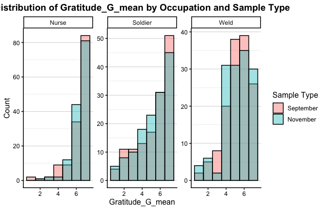
GEN_gratitude_items <- grep("GeneralGratW", names(stacked_num), value = TRUE)
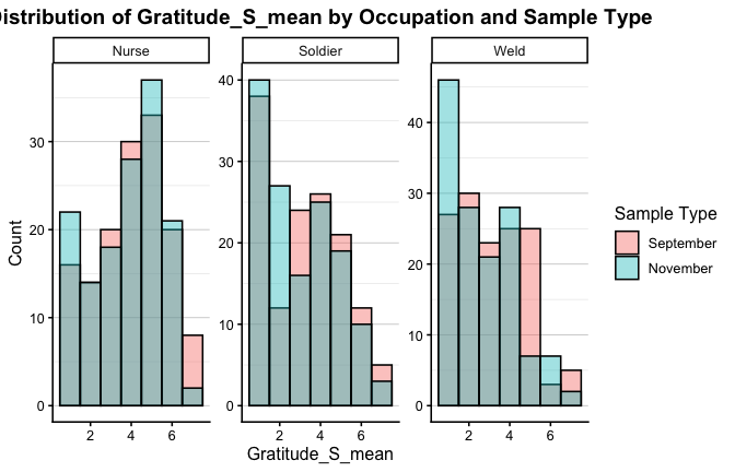
SPEC_gratitude_items <- grep("SpecGratW", names(stacked_num), value = TRUE)
## 3 factors: 1 clear general with only the 3 first that are good:
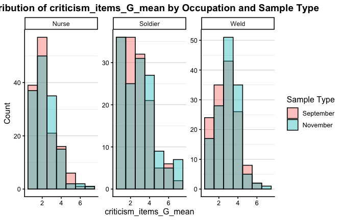
criticism_items_G <- grep("GenCritW", names(stacked_num), value = TRUE)
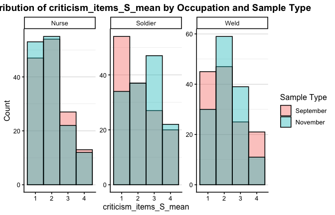
# Only the 'chill' posts are good. the two extreme ones measuring something else.
criticism_items_S <- grep("severity", names(stacked_num), value = TRUE)
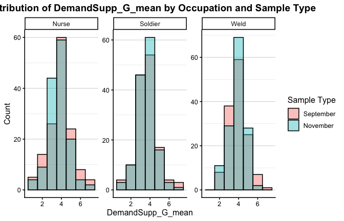
# Let's keep the General that is distinct from specific (focus on protesting)
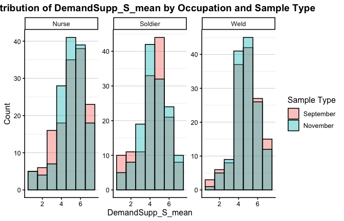
DemandSupp_G <- grep("GenSuppW", names(stacked_num), value = TRUE)
DemandSupp_S <- grep("SpecSuppW", names(stacked_num), value = TRUE)
# General works fine
Victim_G <- grep("GenVictW", names(stacked_num), value = TRUE)
# Same for Specific
Victim_S <- grep("SpecVictimW", names(stacked_num), value = TRUE)
# Here also: general works fine
Villain_G <- grep("GenImpW", names(stacked_num), value = TRUE)
## But specific not so much...
Villain_S <- grep("SpecImpW", names(stacked_num), value = TRUE)
scales <- list(
Gratitude_G = GEN_gratitude_items,
Gratitude_S = SPEC_gratitude_items,
criticism_items_G = criticism_items_G,
criticism_items_S = criticism_items_S,
DemandSupp_G = DemandSupp_G,
DemandSupp_S = DemandSupp_S,# Only 2 items
Victim_G = Victim_G ,
Victim_S = Victim_S,
Villain_G = Villain_G,
Villain_S = Villain_S
)
for (name in names(scales)) {
items <- scales[[name]]
df_subset <- stacked_num[items]
stacked_num[[paste0(name, "_mean")]] <- rowMeans(df_subset, na.rm = TRUE)
}
colnames(stacked_num)
##  [1] "dataset"                "prolID"                 "SpecGratW_1"
##  [4] "SpecGratW_2"            "SpecGratW_3"            "GeneralGratW"
##  [7] "GenCritW_1"             "GenCritW_2"             "GenCritW_3"
## [10] "SpecCritW1_1"           "SpecCritW1_2"           "SpecCritW1_3"
## [13] "SpecCritW1_9"           "SpecCritW1_4"           "SpecCritW2_1"
## [16] "SpecCritW2_2"           "SpecCritW2_3"           "SpecCritW2_9"
## [19] "SpecCritW2_4"           "SpecSuppW_1"            "SpecSuppW_3"
## [22] "GenVictW_1"             "GenVictW_2"             "GenVictW_3"
## [25] "SpecVictimW_1"          "SpecVictimW_2"          "SpecVictimW_3"
## [28] "GenImpW_1"              "GenImpW_2"              "GenImpW_4"
## [31] "SpecImpW_2"             "SpecImpW_3"             "SpecImpW_4"
## [34] "GenSuppW_1"             "GenSuppW_2"             "HW_1"
## [37] "DangerHelpW_1"          "DangerHelpW_2"          "AttW"
## [40] "Cond"                   "age"                    "SpecCritW1_severity"
## [43] "SpecCritW2_severity"    "Gratitude_G_mean"       "Gratitude_S_mean"
## [46] "criticism_items_G_mean" "criticism_items_S_mean" "DemandSupp_G_mean"
## [49] "DemandSupp_S_mean"      "Victim_G_mean"          "Victim_S_mean"
## [52] "Villain_G_mean"         "Villain_S_mean"
#scale_scores <- stacked_num[, c(40, 2, 48:57, 36:39, 34, 35)]
scale_scores <- stacked_num
scale_scores$Cond <- as.factor(scale_scores$Cond)
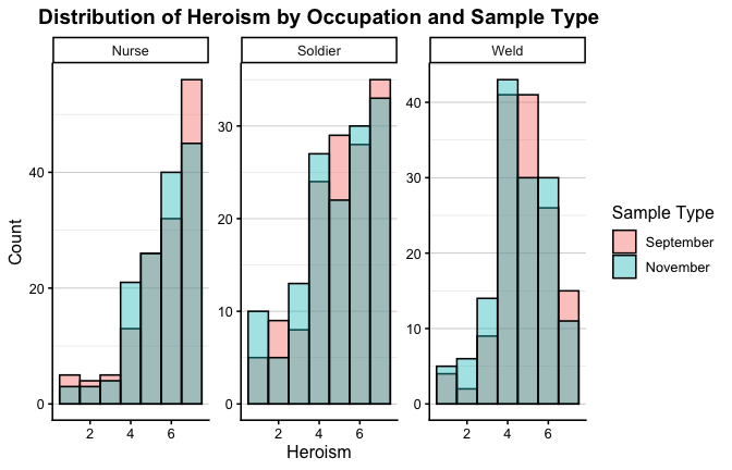
scale_scores$Heroism <- scale_scores$HW_1
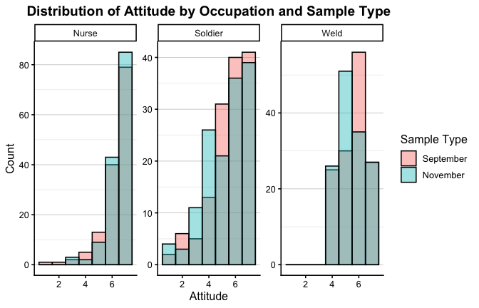
scale_scores$Attitude <- (scale_scores$AttW)
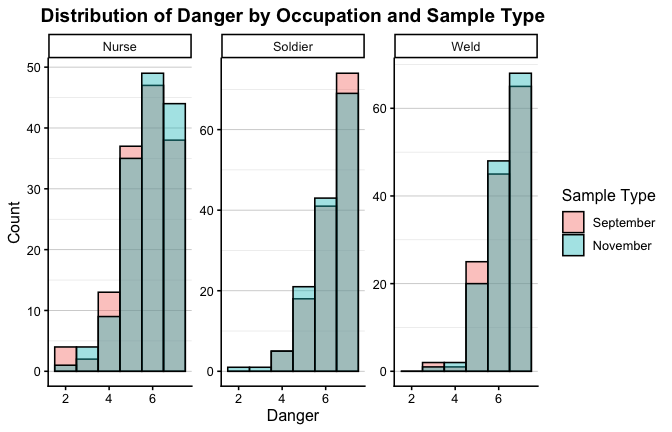
scale_scores$Danger <- (scale_scores$DangerHelpW_1)
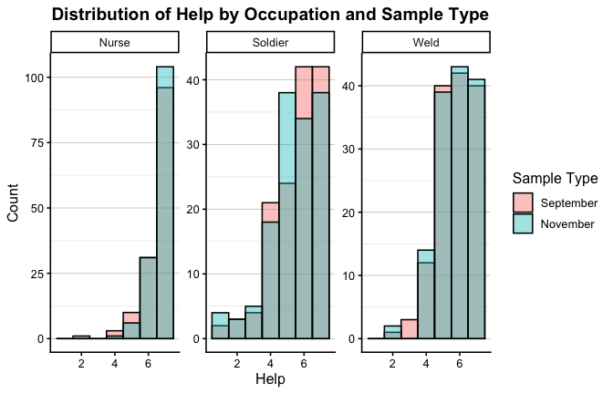
scale_scores$Help <- (scale_scores$DangerHelpW_2)
Poppy1_DF <- subset(scale_scores, scale_scores$Cond == "Soldier")
scale_scores <- subset(scale_scores,
scale_scores$Cond == "Soldier" |
scale_scores$Cond == "Nurse" |
scale_scores$Cond == "Weld")
contrasts(scale_scores$Cond) <- contr.sum(nlevels(scale_scores$Cond))
contrasts(scale_scores$Cond) #
##             [,1] [,2] [,3] [,4] [,5]
## Firefighter    1    0    0    0    0
## Journalist     0    1    0    0    0
## Nurse          0    0    1    0    0
## Psych          0    0    0    1    0
## Soldier        0    0    0    0    1
## Weld          -1   -1   -1   -1   -1
scale_scores$Cond <- droplevels(scale_scores$Cond)
November sample:
DF <- read.csv("~/Downloads/Poppy+Part+2+revised+-+Hero+Project_November+7,+2025_06.33.csv", comment.char="#")
DF <- subset(DF, DF$age != "")
#colnames(DF)
Demographics2 <- DF[-c(1:2), c(150:160)]
DF <- DF[-c(1:2), c(23, 26:45, 50:149, 162, 163, 152)]

#prolOK <- read.csv("Prolific_Export_C1.csv")

#AwaitR<- subset(prolOK, prolOK$Status == "APPROVED")

#DF <- subset(DF, DF$prolID != setdiff(DF$prolID, AwaitR$Participant.id))


Nurs <- subset(DF, DF$Cond == "Nurse")
Nurs <- Nurs[, colSums(!is.na(Nurs) & Nurs != "") > 0 | grepl("SpecCritN", names(Nurs)), drop = FALSE]


Soldier <- subset(DF, DF$Cond == "Soldier")
Soldier <- Soldier[, colSums(!is.na(Soldier) & Soldier != "") > 0 | grepl("SpecCritS", names(Soldier)), drop = FALSE]

Weld <- subset(DF, DF$Cond == "Weld")
Weld <- Weld[, colSums(!is.na(Weld) & Weld != "") > 0 | grepl("SpecCritW", names(Weld)), drop = FALSE]


# 1) Use Weld as the "template" for column names
template_names <- names(Weld)  # 47 names

# 2) Helper that renames a data frame by POSITION to match Weld
rename_like_weld <- function(df, template = template_names) {
  # Sanity checks to avoid silent disasters
  if (ncol(df) != length(template)) {
    stop("Column count mismatch: this df has ", ncol(df),
         " columns but template has ", length(template), ".")
  }
  # Copy names by position
  names(df) <- template
  df
}

# 3) Put all your data frames into a named list
dfs <- list(
  Weld    = Weld,
  Nurs    = Nurs,
  Soldier = Soldier
)

# 4) Harmonise names, then stack vertically with a source column
stacked <- dfs %>%
  purrr::map(rename_like_weld) %>%          # harmonise titles to Weld's names
  bind_rows(.id = "dataset")         # adds the dataset name as the first column

# Result: 48 columns total (1 "dataset" + 47 harmonised vars)
# and nrow(stacked) == sum(nrow(.) for each df)


#------------------------------------------------------------
# 0) Small helpers
#------------------------------------------------------------

# Replace "" and pure whitespace with NA
na_empty <- function(x) {
  x <- if (is.character(x)) str_trim(x) else x
  ifelse(is.character(x) & x == "", NA, x)
}

# Map character -> numeric using a named vector `key`.
# Unknown labels become NA (so you’ll notice and can fix the key).
map_to_num <- function(x, key) {
  x <- na_empty(x)
  # exact match after trimming
  out <- unname(key[ match(x, names(key)) ])
  # if x is already numeric-like (e.g., "5"), keep it
  suppressWarnings({
    out_numlike <- as.numeric(x)
  })
  out[is.na(out) & !is.na(out_numlike)] <- out_numlike[is.na(out) & !is.na(out_numlike)]
  as.numeric(out)
}

# Pull the first integer in a string like "7 - Strongly agree" -> 7
first_int <- function(x) {
  x <- na_empty(x)
  as.numeric(str_extract(x, "\\d+"))
}

# Checkbox columns: any non-empty text -> 1, blank/NA -> 0
checkbox01 <- function(x) as.numeric(!is.na(na_empty(x)))


#------------------------------------------------------------
# 1) Define your scale keys (edit here if wording differs)
#------------------------------------------------------------

agree7 <- c(
  "Strongly disagree"             = 1,
  "Moderately disagree"           = 2,
  "Slightly disagree"             = 3,
  "Neither disagree, nor agree"   = 4,
  "Slightly agree"                = 5,
  "Moderately agree"              = 6,
  "Strongly agree"                = 7
)

likely7 <- c(
  "Very unlikely"                 = 1,
  "Quite unlikely"                = 2,
  "Slightly unlikely"             = 3,
  "Neither likely, nor unlikely"  = 4,
  "Slightly likely"               = 5,
  "Quite likely"                  = 6,
  "Very likely"                   = 7
)

# Frequency (seen in GenSuppDemWeld_*): includes "Always" at the top end
freq7 <- c(
  "Never"            = 1,
  "Very Rarely"      = 2,
  "Rarely"           = 3,
  "Occasionally"     = 4,
  "Frequently"       = 5,
  "Very frequently"  = 6,
  "Always"           = 7
)

# Intensity (seen in GenVictimWeld_*): ordered least -> most
intensity7 <- c(
  "Not at all"   = 1,
  "Very little"  = 2,
  "A little"     = 3,
  "Somewhat"     = 4,
  "Quite a bit"  = 5,
  "A lot"        = 6,
  "Very much"    = 7 #!!!!!

)

# Valence (Q239). Your data shows: Very/Quite negative, Somewhat/Quite/Very positive.
# Map to 1..5 (negative -> positive). If you have "Neither", add it as 3.
valence5 <- c(
  "Very negative"      = 1,
  "Quite negative"            = 2,
  "Somewhat negative"     = 3, #!!!!!!
  "Neutral"  = 4,
  "Somewhat positive"     = 5,
  "Quite positive"      = 6,
  "Very positive" = 7
)

# Gratitude single item (GenGratWeld) appears to use intensity-style words
grat7 <- intensity7


#------------------------------------------------------------
# 2) Identify column groups by name (using your Weld names)
#    We only target cols 2:41, but naming groups is clearer & safer.
#------------------------------------------------------------

agree_cols <- c(
  # Crit accept (general)
  "GenCritW_1","GenCritW_2","GenCritW_3",
  # Specific victims/villains attitudes (agree-type)
  "SpecSuppW_1","SpecSuppW_2","SpecSuppW_3",
  "SpecVictimW_1","SpecVictimW_2","SpecVictimW_3",
  "GenImpW_1","GenImpW_2","GenImpW_3","GenImpW_4",
  "SpecImpW_1","SpecImpW_2","SpecImpW_3","SpecImpW_4"
)

likely_cols <- c("SpecGratW_1","SpecGratW_2","SpecGratW_3")

freq_cols <- c("GenSuppW_1","GenSuppW_2")

intensity_cols <- c("GenVictW_1","GenVictW_2","GenVictW_3","GeneralGratW")

# Checkbox blocks (present/blank -> 1/0)
checkbox_cols <- c(
  "SpecCritW1_1","SpecCritW1_2","SpecCritW1_3","SpecCritW1_9","SpecCritW1_4",
  "SpecCritW2_1","SpecCritW2_2","SpecCritW2_3","SpecCritW2_9","SpecCritW2_4"
)

# Hybrid numeric-label items
hybrid_num_cols <- c("HW_1","DangerHelpW_1","DangerHelpW_2")

# Valence item
valence_cols <- c("AttW")


#------------------------------------------------------------
# 3) Apply mappings to your stacked data (called `stacked`)
#    We leave identifying/meta columns alone: dataset, prolID, gender*, age, Q52, Attentive, Cond
#------------------------------------------------------------

stacked_num <- stacked %>%
  mutate(
    # scales
    across(all_of(agree_cols),    ~ map_to_num(.x, agree7)),
    across(all_of(likely_cols),   ~ map_to_num(.x, likely7)),
    across(all_of(freq_cols),     ~ map_to_num(.x, freq7)),
    across(all_of(intensity_cols),~ map_to_num(.x, intensity7)),
    across(all_of(valence_cols),  ~ map_to_num(.x, valence5)),

    # checkbox-style -> 0/1
    across(all_of(checkbox_cols), checkbox01),

    # hybrid numerics (e.g., "7 - Strongly agree" or just "5")
    across(all_of(hybrid_num_cols), first_int),

    )


colnames(stacked_num)
##  [1] "dataset"       "Q90"           "SpecGratW_1"   "SpecGratW_2"
##  [5] "SpecGratW_3"   "GeneralGratW"  "GenCritW_1"    "GenCritW_2"
##  [9] "GenCritW_3"    "SpecCritW1_1"  "SpecCritW1_2"  "SpecCritW1_3"
## [13] "SpecCritW1_9"  "SpecCritW1_4"  "SpecCritW2_1"  "SpecCritW2_2"
## [17] "SpecCritW2_3"  "SpecCritW2_9"  "SpecCritW2_4"  "SpecSuppW_1"
## [21] "SpecSuppW_2"   "SpecSuppW_3"   "GenVictW_1"    "GenVictW_2"
## [25] "GenVictW_3"    "SpecVictimW_1" "SpecVictimW_2" "SpecVictimW_3"
## [29] "GenImpW_1"     "GenImpW_2"     "GenImpW_3"     "GenImpW_4"
## [33] "SpecImpW_1"    "SpecImpW_2"    "SpecImpW_3"    "SpecImpW_4"
## [37] "GenSuppW_1"    "GenSuppW_2"    "HW_1"          "DangerHelpW_1"
## [41] "DangerHelpW_2" "AttW"          "Attentive"     "Cond"
## [45] "age"
# Remove ATTENTION CHECKS: GenImpW_3 ; SpecSuppW_2; SpecImpW_1
stacked_num <- stacked_num[, -c(21, 31, 33)]


# Severity mapping: column suffix -> numeric severity
severity_map <- c("1" = 1, "2" = 2, "3" = 3, "9" = 4, "4" = 5)

# Helper: collapse one multi-response item (five 0/1 columns) into a single 1..5 severity
most_severe <- function(data, stem, map = severity_map) {
  # Build the expected column names for this stem
  suf  <- names(map)                           # c("1","2","3","9","4")
  cols <- paste0(stem, "_", suf)

  # Safety checks: are all expected columns present?
  missing <- setdiff(cols, names(data))
  if (length(missing)) {
    stop("Missing columns for '", stem, "': ", paste(missing, collapse = ", "))
  }

  # Grab the indicators as a numeric matrix (0/1/NA)
  M <- as.matrix(data[cols])

  # Treat 0 as "not selected" -> NA, so they don't affect the max
  M[M == 0] <- NA

  # Weight each column by its severity value (1..5) so max() = most severe chosen
  sev <- as.numeric(map)
  W   <- sweep(M, 2, sev, `*`)   # column j multiplied by sev[j]

  # Row-wise max ignoring NAs; if all NA -> NA
  out <- apply(W, 1, function(x) {
    m <- suppressWarnings(max(x, na.rm = TRUE))
    if (is.infinite(m)) NA_real_ else m
  })

  # Return as integer 1..5 (or NA if nothing ticked)
  as.integer(out)
}

# Apply to your two stems
stems <- c("SpecCritW1", "SpecCritW2")

for (s in stems) {
  newcol <- paste0(s, "_severity")
  stacked_num[[newcol]] <- most_severe(stacked_num, s)
}

gratitude_items <- grep("GeneralGrat|SpecGrat", names(stacked_num), value = TRUE)
criticism_items <- grep("SpecCritW1_severity|SpecCritW2_severity|GenCrit", names(stacked_num), value = TRUE)
demand_items    <- grep("SpecSupp|GenSupp", names(stacked_num), value = TRUE)
victim_items    <- grep("GenVict|SpecVictim", names(stacked_num), value = TRUE)
violation_items <- grep("GenImp|SpecImp", names(stacked_num), value = TRUE)

# Store all subscales in a named list for looping
scales <- list(
  Gratitude = gratitude_items,
  Criticism = criticism_items,
  Demands = demand_items,
  Victimhood = victim_items,
  Violations = violation_items
)


### Reversing items
stacked_num$SpecVictimW_1<- 8 -stacked_num$SpecVictimW_1

stacked_num$GenSuppW_1<- 8 -stacked_num$GenSuppW_1

stacked_num$GenCritW_1<- 8 -stacked_num$GenCritW_1
stacked_num$GenCritW_2<- 8 -stacked_num$GenCritW_2
stacked_num$GenCritW_3<- 8 -stacked_num$GenCritW_3

stacked_num$SpecCritW1_severity<- 6 -stacked_num$SpecCritW1_severity
stacked_num$SpecCritW2_severity<- 6 -stacked_num$SpecCritW2_severity


### Two, perfectly defined subscale: general vs specific
GEN_gratitude_items <- grep("GeneralGratW", names(stacked_num), value = TRUE)
SPEC_gratitude_items <- grep("SpecGratW", names(stacked_num), value = TRUE)


## 3 factors: 1 clear general with only the 3 first that are good:
criticism_items_G <- grep("GenCritW", names(stacked_num), value = TRUE)
# Only the 'chill' posts are good. the two extreme ones measuring something else.
criticism_items_S <- grep("severity", names(stacked_num), value = TRUE)


# Let's keep the General that is distinct from specific (focus on protesting)
DemandSupp_G <- grep("GenSuppW", names(stacked_num), value = TRUE)


DemandSupp_S <- grep("SpecSuppW", names(stacked_num), value = TRUE)


# General works fine
Victim_G  <- grep("GenVictW", names(stacked_num), value = TRUE)
# Same for Specific
Victim_S  <- grep("SpecVictimW", names(stacked_num), value = TRUE)


# Here also: general works fine

Villain_G  <- grep("GenImpW", names(stacked_num), value = TRUE)

## But specific not so much...
Villain_S <- grep("SpecImpW", names(stacked_num), value = TRUE)


scales <- list(
  Gratitude_G = GEN_gratitude_items,
  Gratitude_S = SPEC_gratitude_items,

  criticism_items_G = criticism_items_G,
  criticism_items_S = criticism_items_S,

  DemandSupp_G  = DemandSupp_G,
  DemandSupp_S = DemandSupp_S,# Only 2 items

  Victim_G  = Victim_G ,
  Victim_S = Victim_S,

  Villain_G = Villain_G,
  Villain_S = Villain_S
)


for (name in names(scales)) {
  items <- scales[[name]]
  df_subset <- stacked_num[items]
  stacked_num[[paste0(name, "_mean")]] <- rowMeans(df_subset, na.rm = TRUE)
}


#colnames(stacked_num)

#scale_scores <- stacked_num[, c(40, 2, 48:57, 36:39, 34, 35)]
scale_scores2 <- stacked_num
scale_scores2$Cond <- as.factor(scale_scores2$Cond)
contrasts(scale_scores2$Cond) <- contr.sum(nlevels(scale_scores2$Cond))
contrasts(scale_scores2$Cond) # Deviations from registration!! We need to use sum to zero contrasts to make coef interpretable
##         [,1] [,2]
## Nurse      1    0
## Soldier    0    1
## Weld      -1   -1
scale_scores2$Heroism <- scale_scores2$HW_1
scale_scores2$Attitude <- (scale_scores2$AttW)
scale_scores2$Danger <- (scale_scores2$DangerHelpW_1)
scale_scores2$Help <- (scale_scores2$DangerHelpW_2)

Poppy2_DF <- subset(scale_scores2, scale_scores2$Cond == "Soldier")

contrasts(scale_scores2$Cond) <- contr.sum(nlevels(scale_scores2$Cond))
contrasts(scale_scores2$Cond)
##         [,1] [,2]
## Nurse      1    0
## Soldier    0    1
## Weld      -1   -1